Beyond PPO - The New Wave of Policy Optimization Techniques for LLM Post-Training

PPO used to be the default workhorse for RLHF because it’s reasonably stable and easy to reason about, but at LLM post-training scale its tradeoffs start to bite: the critic/value model is expensive to train and maintain, long text rollouts amplify variance and make advantage estimation brittle, clipping becomes a blunt instrument that can under-update (wasting samples) or over-update (destabilizing), and the whole loop turns into a systems-heavy exercise once “environment interaction” means generating thousands of tokens across distributed inference. As post-training shifted from short preference tuning toward reasoning-heavy objectives (RLVR, long-CoT, verifier-driven rewards, pass@k-style targets) and larger, more heterogeneous data mixtures, these weaknesses became harder to paper over with hyperparameter folklore because the optimization problem is noisier, the feedback signals are sparser, and the failure modes (reward hacking, length bias, mode collapse, over-regularization) are more punishing. That’s why the field has been moving beyond “just PPO” toward more robust, more LLM-native policy optimization: methods that reduce dependence on a critic, stabilize updates under long-horizon generation, better control distribution shift between samples and policy, and align the training objective with how we actually evaluate modern models, ultimately making post-training not just possible, but reliable under the messy realities of large-scale reasoning optimization.

1) From PPO to GRPO

Proximal Policy Optimization (PPO) is the standard “safe policy gradient” workhorse: you collect trajectories using an old policy $\pi_{\theta_{\text{old}}}$, then update a new policy $\pi_\theta$ to make good actions more likely and bad actions less likely but only by a limited amount per update so training doesn’t blow up. The core trick is the importance ratio:

$$ r_t(\theta)=\frac{\pi_\theta(a_t|s_t)}{\pi_{\theta_{\text{old}}}(a_t|s_t)} $$

which measures how much the new policy changes the probability of the sampled action $a_t$ in state $s_t$, PPO multiplies this by an advantage $\hat A_t$ (how much better that action was than expected, typically estimated using a learned value function/critic $V_Φ$ via GAE) and optimizes a clipped surrogate:

$$ L^{\text{CLIP}}(\theta) = \mathbb{E}_t\left[\min\big(r_t\hat A_t, \text{clip}(r_t,1-\epsilon,1+\epsilon)\hat A_t\big)\right] $$

where the clip parameter $\epsilon$ enforces “don’t move the policy too far” (a trust-region-lite constraint). In practice you train with a combined objective: maximize the clipped policy term, plus a value regression loss $\mathbb{E}_t [(V_Φ)(s_t)-\hat V_t)^2]$ to keep $\hat A_t$ low-variance, and often an entropy bonus to avoid collapse. The full loss optimized in practice (gradient descent) is typically written as:

$$ \mathcal{L}(\theta, Φ)= -L^{\text{CLIP}}(\theta) + c_v \mathbb{E}_t\left[\big(V_Φ(s_t)-\hat V_t\big)^2\right] - c_e \mathbb{E}_t [H (\pi_θ(\cdot\mid s_t)] $$

where:

the first term is the (negative) policy objective,
the second is the value/critic regression loss,
the third is an entropy bonus (encourages exploration / prevents collapse)
$c_v, c_e$ are coefficients.

In RLHF, you usually also keep the policy close to a reference model $\pi_{\text{ref}}$. Often this is implemented as:

either a KL penalty in reward (per token),
or an explicit term in the objective.

A common explicit version: $$ \mathbb{E}_t [β D _ {\text{KL}} (\pi_θ(\cdot\mid s_t) || \pi _ {\text{ref}}(\cdot\mid s_t))] $$

added to the loss (penalizing deviation from reference).

So PPO is essentially policy gradient + baseline + a hard brake on update size to keep learning stable.

PPO became the “default RLHF optimizer” mostly because it’s a pragmatic compromise: it gives you a trust-region-ish update without the full TRPO machinery, and it’s reasonably stable when your policy gradient estimates are noisy. In LLM post-training, though, PPO inherits two pain points that get worse exactly when you care the most (reasoning + long rollouts): (1) the critic tax and (2) mismatch between token-level machinery and sequence-level rewards. DeepSeekMath spells this out bluntly: PPO requires training a value function baseline, which is typically a model comparable in size to the policy, adding substantial memory/compute burden; and in the LLM setting the reward model often assigns a score only at the end, which makes it awkward to train a value function “accurate at each token.”

Let’s make the failure mode concrete. PPO’s core surrogate objective (token-level importance ratios with clipping) looks like: you sample an output $o$ from the old policy $\pi_{\theta_{\text{old}}}$, compute per-token advantages $A_t$ (often via GAE + a learned value $V_\psi$), and optimize a clipped objective to avoid large policy updates.

In “classic RL,” learning a critic is annoying but manageable. In RLHF-for-LLMs, it becomes a constant tax:

You’re basically training an extra LLM (the value model) plus keeping the reference model and reward model around.
Your reward is often sparse / end-of-sequence, but PPO wants token-level advantages; you end up backfilling credit assignment with heuristics (GAE, reward shaping, KL-in-reward, etc.) and now your “algorithm” is half math, half duct tape. DeepSeekMath explicitly notes this tension between end-of-sequence reward scoring and token-wise value modeling.
As sequences get longer, variance rises and the “clip knob” becomes a vibe-based tuning exercise.

2) GRPO: Group Relative Policy Optimization (GRPO)

GRPO keeps the spirit of PPO (importance ratios + clipping + KL regularization), but it swaps out the value function baseline with something you can compute for free from sampling: generate G completions for the same prompt, score them, and use the group’s average as the baseline. DeepSeekMath frames GRPO as “obviating the need for additional value function approximation” and instead using “the average reward of multiple sampled outputs…as the baseline.” That one swap has huge downstream effects:

No critic model to train.
Advantage estimation becomes within-prompt, relative, matching how preference/reward models are often trained (comparisons among outputs for the same question). DeepSeekMath makes this alignment argument explicitly.

DeepSeekMath defines a GRPO objective that still looks PPO-like: for each prompt $q$, sample a group $ {o_i} _ {i=1}^G$ from $ \pi _ {\theta _ {\text{old}}}$, then optimize a clipped surrogate over tokens, plus a KL term to a reference policy. DeepSeek-R1’s report gives a clean, readable version of the same idea at the sequence level:

$$ J _ { \text{GRPO} } ( \theta ) = \mathbb{E} _ { q \sim \mathcal{D} , { o _ i } _ { i = 1 } ^ G \sim \pi _ { \theta _ { \text{old} } } ( \cdot | q ) } $$

$$ [ \frac{1}{G} \sum _ { i = 1 } ^ G \min ( r _ i ( \theta ) A _ i , \text{clip} ( r _ i ( \theta ) , 1 - \epsilon , 1 + \epsilon ) A _ i ) - \beta \mathbb{D} _ { \text{KL} } ( \pi _ \theta ( \cdot | q ) || \pi _ { \text{ref} } ( \cdot | q ) ) ] $$

where:

$$ \underbrace{ \frac{1}{ \color{purple}{G} } \sum _ { i = 1 } ^ { \color{purple}{G} } } _ { \color{purple}{ \text{Group size } G } } ( \min ( \underbrace{ \color{blue}{ \frac{ \pi _ \theta ( o _ i | q ) }{ \pi _ { \theta _ { \text{old} } } ( o _ i | q ) } } } _ { \color{blue}{ \text{probability ratio} } } \underbrace{ \color{magenta}{ A _ i } } _ { \color{magenta}{ \text{advantage} } } , \underbrace{ \color{red}{ \text{clip} ( \color{blue}{ \frac{ \pi _ \theta ( o _ i | q ) }{ \pi _ { \theta _ { \text{old} } } ( o _ i | q ) } } , 1 - \epsilon , 1 + \epsilon ) } } _ { \color{red}{ \text {clipping keeps ratio in }[1-\epsilon,1+\epsilon] } } \underbrace{ \color{magenta}{ A _ i } } _ { \color{magenta}{ \text{advantage} } } ) - \underbrace{ \color{orange}{ \beta \mathbb{D} _ { \text{KL} } ( \pi _ \theta || \pi _ { \text{ref} } ) } } _ { \color{orange}{ \text{KL penalty} } } ) $$

$$ \color{purple}{ \epsilon , \beta \text{ are hyperparameters.} } $$

$$ \color{magenta}{ A _ i } = \frac{ \color{magenta}{ r _ i } - \text{mean} ( { \color{magenta}{ r _ 1 } , \color{magenta}{ r _ 2 } , \dots , \color{magenta}{ r _ G } } ) }{ \text{std} ( { \color{magenta}{ r _ 1 } , \color{magenta}{ r _ 2 } , \dots , \color{magenta}{ r _ G } } ) } $$

$$ \color{magenta}{ \text{(how much better/worse } o _ i \text{ is vs the group baseline).} } $$

GRPO turns advantage estimation into a local ranking problem. Each prompt produces a small batch of candidates; the reward model (or verifier) scores them; and the policy update says “increase probability of better-than-average completions, decrease probability of worse-than-average ones,” while clipping prevents the model from overreacting to a noisy batch.

Let’s understand some of the key terms from the above objective function:

The Importance Weight: A key ingredient in GRPO is the importance weight: a per-token quantity that tells us how much the current policy has changed its mind compared to the old policy. Intuitively, it answers: “Is token $o_{i,t}$ more likely or less likely under the updated model than it was when we generated the sample?” This matters because GRPO (like PPO) learns from data generated by an earlier snapshot of the policy, so we need a way to correct for that mismatch. Formally, consider the $t$-th token of the $i$-th sampled completion, $o_{i,t}$. The token is conditioned on the prompt $q$ and the previously generated tokens $o_{i,<t}$. The importance weight is the ratio of the token’s probability under the current policy $\pi_\theta$ to its probability under the old policy $\pi_{\theta_{\text{old}}}$:
$$ w_{i,t}(\theta)=\frac{\pi_\theta \left(o_{i,t}\mid q, o_{i,<t}\right)}{\pi_{\theta_{\text{old}}} \left(o_{i,t}\mid q ,o_{i,<t}\right)}. $$
If $w_{i,t}(\theta) > 1$, the new policy assigns higher probability to that token than the old policy did; if $w_{i,t}(\theta) < 1$, it assigns lower probability. In other words, this ratio is a direct measure of how strongly the update is pushing the model toward (or away from) specific token choices within a generated answer.
The Advantage Term $A_i$: Once GRPO has a group of $G$ sampled completions for the same prompt $q$, it needs a learning signal that says which samples are worth reinforcing. That’s what the advantage $A_i$ does: it measures how much better (or worse) a particular completion $o_i$is relative to the other completions in the same group. Think of it as a tiny “local ranking” step: for a given question, you generate multiple answers, score them with a reward signal (reward model / verifier / rule-based checker), and then ask: “Is this answer above average for this prompt?” If yes, $A_i$ is positive and GRPO increases its probability; if no, $A_i$ is negative and GRPO suppresses it. This is the core GRPO trick: you get a baseline for free from the group itself, instead of training a separate critic/value model like PPO. In practice, GRPO typically uses a normalized, group-centered reward:
$$ A _ i = \frac{ R _ i - \text{mean} ( { R _ 1 , R _ 2 , \dots , R _ G } ) }{ \text{std} ( { R _ 1 , R _ 2 , \dots , R _ G } ) } $$
where: i) $R_i$ - is the reward score for completion $o_i$. ii) $\operatorname{mean}(⋅)$ - is the average reward across the group (the baseline). iii) $\operatorname{std}(⋅)$ - rescales by the group’s spread, making updates less sensitive to the absolute scale of rewards.
The Clipping Term: GRPO borrows PPO’s most important stability trick: clipping the importance ratio so each update stays proximal to the policy that generated the samples. Without clipping, the optimizer can “overreact” to a high-reward sample by massively increasing its probability in a single step, especially when rewards are noisy (which they often are in LLM post-training). The object being clipped is the importance ratio (sequence-level or token-level). Clipping forces it into a tight band around 1: $$ \text{clip} ( r ( \theta ) , 1 - \epsilon , 1 + \epsilon ) $$

Key changes vs PPO

Critic-free baseline: PPO’s $A_t$ comes from GAE + value model; GRPO’s advantage comes from the group’s relative scores. This is the resource and complexity win DeepSeekMath emphasizes.
Relative (within-prompt) learning signal: Instead of asking for an absolute, token-wise value prediction, you use “how did this completion do compared to siblings for the same prompt,” which is closer to how reward models are trained (pairwise comparisons).
KL handling becomes cleaner: DeepSeekMath notes that rather than folding KL into the reward (per-token KL penalty inside $r_t$ in PPO-style RLHF), GRPO adds KL divergence directly to the loss, which avoids complicating advantage calculation.

3) DR.GRPO (GRPO done Right)

GRPO is a big step up from PPO in practice, but its default objective quietly smuggles in biases:

Baseline bias (group mean scaling): In GRPO, the advantage is built by subtracting a group baseline, typically the average reward (or score) over the $G$ sampled completions for the same prompt. The subtle issue is that if you treat the group mean as the baseline for each sample, the “right” way to scale that baseline is tied to the fact that each sample is being compared against the other $G-1$ samples, not against a population mean. Using a naive $\frac{1}{G}$ scaling instead of the correct $\frac{1}{G-1}$ style correction introduces a small but systematic mis-scaling of the advantage, which means the GRPO gradient is biased even before clipping or KL come into play.
Response-level length bias ($\mathbf{1/|o_i|}$ factor): Many GRPO implementations average the token-level surrogate by response length via a factor $\frac{1}{|o_i|}\sum_{t}\cdots$. In the GRPO objective, that turns the same sequence-level advantage into a per-token learning rate that depends on how long the model chose to talk. The consequence is asymmetric: for positive advantage samples (usually correct/high-reward answers), the update is stronger when the response is shorter (reward is concentrated into fewer tokens), so GRPO implicitly prefers short correct answers; for negative advantage samples (often incorrect answers), the penalty is diluted when the response is longer, so the model can “hide” badness by generating more tokens. This is exactly the “short correct, long wrong” failure pattern that motivates Dr. GRPO.
Question-level difficulty bias (std-normalized advantages): GRPO often normalizes advantages within each prompt’s group, e.g. $\hat A_i = \frac{R_i-\text{mean}(R)}{\text{std}(R)}$. That sounds like harmless variance reduction, but in the GRPO objective it effectively reweights prompts based on their within-group reward spread. Since different prompts vary widely in domain and difficulty (LLM post-training is effectively multi-task RL), prompts with low reward variance (often very easy or very hard prompts where all sampled answers score similarly) get their gradients amplified by dividing by a small std, while prompts with higher variance get damped. This distorts the learning signal across prompts: instead of naturally focusing on medium-difficulty questions (where learning is most productive), the std term can unintentionally upweight easy and impossible prompts, pushing GRPO’s optimization in a less efficient direction.

For the baseline-bias issue, the mismatch is essentially just a constant rescaling of the gradient, which you can fold into the effective learning rate. And since practitioners tune the learning rate anyway, this particular bias typically has little to no noticeable impact on final training performance. For the other two biases, Group Relative Policy Optimization Done Right (Dr. GRPO) addresses them by simply removing $1/∣o∣$ and $std⁡[r_k]$:

$$ \textbf{GRPO} $$

$$ \qquad \frac{1}{G} \sum _ { i = 1 } ^ G {\color{red}{ \frac{1}{ | o _ i | } }} \sum _ { t = 1 } ^ { | o _ i | } { \min [ \frac{ \pi _ \theta ( o _ { i,t } | q , o _ { i,<t } ) }{ \pi _ { \theta _ { \text{old} } } ( o _ { i,t } | q , o _ { i,<t } ) } \hat{A} _ { i,t } , \text{clip} ( \frac{ \pi _ \theta ( o _ { i,t } | q , o _ { i,<t } ) }{ \pi _ { \theta _ { \text{old} } } ( o _ { i,t } | q , o _ { i,<t } ) } , 1 - \epsilon , 1 + \epsilon ) \hat{A} _ { i,t } ] } $$

$$ \text{where} \quad \hat{A} _ { i,t } = \frac{ R ( q , o _ i ) - \text{mean} ( { R ( q , o _ 1 ) , \dots , R ( q , o _ G ) } ) }{ \color{red}{ \text{std} ( { R ( q , o _ 1 ) , \dots , R ( q , o _ G ) } ) } } $$

$$ \textbf{Dr. GRPO} \quad \text{(GRPO Done Right, without bias)} $$

$$ \qquad \frac{1}{G} \sum _ { i = 1 } ^ G \sum _ { t = 1 } ^ { | o _ i | } { \min [ \frac{ \pi _ \theta ( o _ { i,t } | q , o _ { i, <t } ) }{ \pi _ { \theta _ { \text{old} } } ( o _ { i,t } | q , o _ { i, <t } ) } \hat{A} _ { i,t } , \text{clip} ( \frac{ \pi _ \theta ( o _ { i,t } | q , o _ { i, <t } ) }{ \pi _ { \theta _ { \text{old} } } ( o _ { i,t } | q , o _ { i, <t } ) } , 1 - \epsilon , 1 + \epsilon ) \hat{A} _ { i,t } ] } $$

$$ \text{where} \quad \hat{A} _ { i,t } = R ( q , o _ i ) - \text{mean} ( { R ( q , o _ 1 ) , \dots , R ( q , o _ G ) } ) $$

By correcting these mathematical inconsistencies, Dr. GRPO prevents the “double-increase” phenomenon where response lengths grow uncontrollably, enhances token efficiency, and reduces the tendency for “overthinking” in incorrect responses while consistently achieving superior accuracy and training stability compared to vanilla GRPO.

4) GSPO (Group Sequence Policy Optimization)

GRPO inherits PPO’s off-policy correction instinct, but it pushes it down to the token level: every next-token decision gets its own importance-sampling ratio, even though we only observed one sample from that conditional distribution. In proper IS, the ratio earns its keep by averaging over many samples from the behavior policy; here, the “correction” mostly acts like a noisy multiplicative weight on the gradient. The GSPO authors argue this is the wrong granularity for LLM post-training: the variance from token-wise ratios compounds across long responses, and once you add clipping on top, you can end up amplifying the worst kinds of noise, creating training dynamics that don’t just wobble, but can collapse catastrophically and sometimes never recover.

Group Sequence Policy Optimization (GSPO) is essentially a “unit fix”: it moves the core optimization step from tokens to sequences, and that shift is what buys stability. The motivation is straightforward, prior group-based methods like GRPO can become unstable on long-reasoning, large-scale training, sometimes spiraling into a collapse that doesn’t recover. GSPO tackles this in a few concrete ways.

First, it corrects what the authors describe as a misuse of importance sampling in GRPO: GRPO applies an IS-style weight at every token position, but that weight is computed from a single sampled token, which doesn’t serve the variance-reduction role IS is supposed to play; instead it injects noisy multiplicative factors into the gradient and that noise compounds with response length. GSPO replaces this with a sequence-level importance ratio $s_i$ based on whole-sequence likelihood, matching the fact that the reward signal is typically assigned to the entire completion, not individual tokens.

Second, the gradient structure becomes much cleaner: GRPO effectively reweights tokens unequally via token-level ratios $w_{i,t}$, which can swing wildly and destabilize updates; GSPO gives all tokens in a response equal weight and applies the correction once per sequence, removing a major source of jitter.

Third, this matters a lot for Mixture-of-Experts: MoE routing can change sharply after a single update, making token-level ratios extremely volatile (and forcing hacks like “routing replay” in GRPO-style training), whereas sequence likelihood remains comparatively stable even when internal expert choices shift, so GSPO can train MoE models without those artificial constraints. Finally, GSPO clips at the response level rather than token level, which cleanly drops overly off-policy sequences from contributing to the update, and it uses length-normalized sequence ratios so responses of different lengths live in a comparable numerical range.

Token-level ratio: $$ \frac{\pi_\theta(y_{i,t}\mid x,y_{i,<t})}{\pi_{\theta_{\text{old}}}(y_{i,t}\mid x,y_{i,<t})} $$ can be extremely noisy and unstable when applied per token.

Sequence-level ratio: $$ \frac{\pi_\theta(y_i\mid x)}{\pi_{\theta_{\text{old}}}(y_i\mid x)} $$
directly answers: “How much more likely is the whole sampled response under the new policy than under the old policy?” That matches how LLM rewards are usually defined: reward is assigned to the whole response.

GSPO employs the following sequence-level optimization objective:

$$ \mathcal{J} _ { \text{GSPO} } ( \theta ) = \mathbb{E} _ { x \sim D , { y _ i } _ { i = 1 } ^ G \sim \pi _ { \theta _ { \text{old} } } ( \cdot | x ) } $$

$$ [ \frac{1}{G} \sum _ { i = 1 } ^ G \min ( s _ i ( \theta ) \hat{A} _ i , \text{clip} ( s _ i ( \theta ) , 1 - \epsilon , 1 + \epsilon ) \hat{A} _ i ) ] $$

where,

$$ \hat{A} _ i = \frac{ r ( x , y _ i ) - \text{mean} ( { r ( x , y _ j ) } _ { j = 1 } ^ G ) }{ \text{std} ( { r ( x , y _ j ) } _ { j = 1 } ^ G ) } $$

and the sequence-level importance ratio:

$$ s _ i ( \theta ) = \left( \frac{ \pi _ \theta ( y _ i | x ) }{ \pi _ { \theta _ { \text{old} } } ( y _ i | x ) } \right) ^ { \frac{1}{ | y _ i | } } = \exp \left( \frac{1}{ | y _ i | } \sum _ { t = 1 } ^ { | y _ i | } \log \frac{ \pi _ \theta ( y _ { i,t } | x , y _ { i, <t } ) }{ \pi _ { \theta _ { \text{old} } } ( y _ { i,t } | x , y _ { i, <t } ) } \right) $$

$\pi_\theta(y_i\mid x)=\prod_t \pi_\theta(y_{i,t}\mid x,y_{i,<t})$ is the likelihood of the full response.
The raw ratio $\pi_\theta(y_i\mid x)/\pi_{\text{old}}(y_i\mid x)$ can explode/vanish for long sequences (product of many factors).
So they take the geometric mean per token ($1/|y_i|$ exponent), keeping $s_i(\theta)$ in a stable numeric range and making clipping comparable across different lengths.
Also: GSPO clips at the response level, i.e., it drops overly off-policy responses rather than clipping token-by-token.

Gradient of GSPO:

$$ \nabla _ \theta \mathcal{J} _ { \text{GSPO} } ( \theta ) = \nabla _ \theta \mathbb{E} _ { x \sim D , { y _ i } _ { i = 1 } ^ G \sim \pi _ { \theta _ { \text{old} } } ( \cdot | x ) } \left[ \frac{1}{G} \sum _ { i = 1 } ^ G s _ i ( \theta ) \hat{A} _ i \right] $$

$$ = \mathbb{E} _ { x \sim D , { y _ i } _ { i = 1 } ^ G \sim \pi _ { \theta _ { \text{old} } } ( \cdot | x ) } \left[ \frac{1}{G} \sum _ { i = 1 } ^ G s _ i ( \theta ) \hat{A} _ i \cdot \nabla _ \theta \log s _ i ( \theta ) \right] $$

$$ = \mathbb{E} _ { x \sim D , { y _ i } _ { i = 1 } ^ G \sim \pi _ { \theta _ { \text{old} } } ( \cdot | x ) } \left[ \frac{1}{G} \sum _ { i = 1 } ^ G \left( \frac{ \pi _ \theta ( y _ i | x ) }{ \pi _ { \theta _ { \text{old} } } ( y _ i | x ) } \right) ^ { \frac{1}{ | y _ i | } } \hat{A} _ i \cdot \frac{1}{ | y _ i | } \sum _ { t = 1 } ^ { | y _ i | } \nabla _ \theta \log \pi _ \theta ( y _ { i,t } | x , y _ { i, <t } ) \right] $$

Gradient of GRPO:

$$ \nabla _ \theta \mathcal{J} _ { \text{GRPO} } ( \theta ) = \nabla _ \theta \mathbb{E} _ { x \sim D , { y _ i } _ { i = 1 } ^ G \sim \pi _ { \theta _ { \text{old} } } ( \cdot | x ) } [ \frac{1}{G} \sum _ { i = 1 } ^ G \frac{1}{ | y _ i | } \sum _ { t = 1 } ^ { | y _ i | } w _ { i,t } ( \theta ) \hat{A} _ { i,t } ] $$

$$ = \mathbb{E} _ { x \sim D , { y _ i } _ { i = 1 } ^ G \sim \pi _ { \theta _ { \text{old} } } ( \cdot | x ) } [ \frac{1}{G} \sum _ { i = 1 } ^ G \hat{A} _ i \cdot \frac{1}{ | y _ i | } \sum _ { t = 1 } ^ { | y _ i | } \frac{ \pi _ \theta ( y _ { i,t } | x , y _ { i, <t } ) }{ \pi _ { \theta _ { \text{old} } } ( y _ { i,t } | x , y _ { i, <t } ) } \nabla _ \theta \log \pi _ \theta ( y _ { i,t } | x , y _ { i, <t } ) ] $$

GSPO-token: token-wise advantages without token-wise IS instability

GSPO-token is introduced for scenarios where the sequence-level advantage $\hat A_i$ is too coarse, multi-turn RL is the canonical example, so you want the flexibility to assign token-specific advantages $\hat A_{i,t}$. The danger is that if you naïvely go token-level again, you risk reintroducing GRPO’s token-level importance weight problems. GSPO-token avoids that by using a clever stop-gradient (detach) construction for $s_{i,t}(\theta)$: numerically, $s_{i,t}$ equals the same sequence-level ratio $s_i$, but the gradient is arranged so you still get GSPO-like stable behavior (sequence-level weighting) while allowing per-token advantage shaping. The paper notes an important sanity check: if you set $\hat A_{i,t}=\hat A_i$ for all tokens, then GSPO-token and GSPO become essentially identical (same objective value, same clipping behavior, and the same theoretical gradient). The only difference is that GSPO-token gives you an extra degree of freedom when you do want $\hat A_{i,t}$ to vary across tokens.

$$ \mathcal{J} _ { \text{GSPO-token} } ( \theta ) = \mathbb{E} _ { x \sim D , { y _ i } _ { i = 1 } ^ G \sim \pi _ { \theta _ { \text{old} } } ( \cdot | x ) } $$

$$ \left[ \frac{1}{G} \sum _ { i = 1 } ^ G \frac{1}{ | y _ i | } \sum _ { t = 1 } ^ { | y _ i | } \min ( s _ { i,t } ( \theta ) \hat{A} _ { i,t } , \text{clip} ( s _ { i,t } ( \theta ) , 1 - \epsilon , 1 + \epsilon ) \hat{A} _ { i,t } ) \right] $$

$$ s _ { i,t } ( \theta ) = \text{sg} [ s _ i ( \theta ) ] \cdot \frac{ s _ i ( \theta ) }{ \text{sg} [ s _ i ( \theta ) ] } $$

Here $\operatorname{sg}[\cdot]$ means stop gradient (PyTorch detach()): it keeps the numerical value but blocks backprop through that term.

5) Decoupled Clip and Dynamic Sampling Policy Optimization (DAPO)

GRPO is a great baseline for “critic-free RL,” but once you push it into long-CoT, high-variance, large-scale post-training, it starts to show very practical cracks: batches with almost no learning signal (everyone in the group is either correct or wrong), clipping that quietly strangles exploration, loss reductions that underweight long trajectories (letting repetition/length pathologies slip through) and reward noise introduced by truncation at max length.

DAPO samples a group of outputs ${o_i}_{i=1}^{G}$ for each question $q$ paired with the answer $a$, and optimizes the policy via the following objective:

$$ \mathcal{J} _ { \text{DAPO} } ( \theta ) = \mathbb{E} _ { ( q , a ) \sim \mathcal{D} , { o _ i } _ { i = 1 } ^ G \sim \pi _ { \theta _ { \text{old} } } ( \cdot | q ) } \left[ \frac{1}{ \sum _ { i = 1 } ^ G | o _ i | } \sum _ { i = 1 } ^ G \sum _ { t = 1 } ^ { | o _ i | } \min ( r _ { i,t } ( \theta ) \hat{A} _ { i,t } , \text{clip} ( r _ { i,t } ( \theta ) , 1 - \epsilon _ { \text{low} } , 1 + \epsilon _ { \text{high} } ) \hat{A} _ { i,t } ) \right] $$

$ s.t 0 < |({o_i | \ is \ equivalent \ (a, o_i )})| < G $

$$ \text{where} \quad r _ { i,t } ( \theta ) = \frac{ \pi _ \theta ( o _ { i,t } | q , o _ { i, <t } ) }{ \pi _ { \theta _ { \text{old} } } ( o _ { i,t } | q , o _ { i, <t } ) } , \qquad \hat{A} _ { i,t } = \frac{ R _ i - \text{mean} ( { R _ i } _ { i = 1 } ^ G ) }{ \text{std} ( { R _ i } _ { i = 1 } ^ G ) } $$

DAPO introduces four primary techniques to stabilize and enhance large-scale RL training:

1) Clip-Higher / decoupled clipping:

One of the easiest ways GRPO-style training goes wrong is entropy collapse: the policy becomes confident too quickly, generations across a group start looking nearly identical, and learning slows down because there’s no diversity left to compare. Standard PPO/GRPO clipping is a trust-region guardrail, but it’s also a blunt instrument: the usual symmetric bound $1-\epsilon, 1+\epsilon$ caps how much the policy can increase probabilities in a single update. That cap matters most for the tokens you actually need to amplify, rare “exploration” moves in long reasoning traces, because they start at tiny probability and require meaningful uplift to show up in sampling.

Clip-Higher fixes this by decoupling the clip bounds: keep the lower bound conservative (so you don’t aggressively squash probabilities to zero), but raise the upper bound to give the optimizer more room to increase low-probability tokens. In practice, that simple asymmetry increases entropy and keeps the sampling space open longer, making group-based learning more effective on long-horizon reasoning.

$$ \mathcal{J} _ { \text{DAPO} } ( \theta ) = \mathbb{E} _ { ( q , a ) \sim \mathcal{D} , { o _ i } _ { i = 1 } ^ G \sim \pi _ { \theta _ { \text{old} } } ( \cdot | q ) } $$

$$ [ \frac{1}{ \sum _ { i = 1 } ^ G | o _ i | } \sum _ { i = 1 } ^ G \sum _ { t = 1 } ^ { | o _ i | } \min ( r _ { i,t } ( \theta ) \hat{A} _ { i,t } , \text{clip} ( r _ { i,t } ( \theta ) , 1 - {\color{red}{ \epsilon _ { \text{low} } }} , 1 + {\color{red}{ \epsilon _ { \text{high} } }} ) \hat{A} _ { i,t } ) ] $$

$ s.t \ 0 < |({o_i | \ is \ equivalent \ (a, o_i )})| < G $

$r_{i,t}(\theta)=\dfrac{\pi_\theta(o_{i,t}\mid q,o_{i,<t})}{\pi_{\theta_{\text{old}}}(o_{i,t}\mid q,o_{i,<t})}$ : token-level importance ratio.
$\hat A_{i,t}$: (group-based) advantage signal copied across tokens of $o_i$.
$\color{red}ε_{high}$: the raised ceiling for probability increases (helps exploration).
$\color{red}{\varepsilon_{\mathrm{low}}}$: kept small to avoid collapsing probability mass by over-penalizing decreases.

2) Dynamic Sampling:

Dynamic sampling is DAPO’s answer to a very specific GRPO failure mode: some prompts stop producing gradients (gradient-decreasing problem). In group-based objectives, the advantage for a prompt is computed relative to the other samples in the same group. If all $G$ sampled outputs for a prompt are correct (accuracy =1) and receive essentially the same reward, then every sample looks identical relative to the group baseline, so the advantage collapses to ~0. Once $\hat A \approx 0$, the whole prompt contributes almost no policy gradient. As training progresses, more prompts become “too easy” (all correct) or “too hard” (all wrong), so an increasing fraction of your batch becomes ineffective—gradient magnitude shrinks and noise dominates.

Dynamic sampling fixes this by over-sampling and filtering: keep drawing samples until you build groups where the prompt has some correct and some incorrect responses, i.e., the group has contrast. That guarantees non-trivial advantages and keeps a stable number of “effective prompts” per batch.

The objective stays the same; the key addition is the constraint that the number of correct/equivalent samples is neither 0 nor $G$:

$$ \mathcal{J} _ { \text{DAPO} } ( \theta ) = \mathbb{E} _ { ( q , a ) \sim \mathcal{D} , { o _ i } _ { i = 1 } ^ G \sim \pi _ { \theta _ { \text{old} } } ( \cdot | q ) } $$

$$ \left[ \frac{1}{ \sum _ { i = 1 } ^ G | o _ i | } \sum _ { i = 1 } ^ G \sum _ { t = 1 } ^ { | o _ i | } \min ( r _ { i,t } ( \theta ) \hat{A} _ { i,t } , \text{clip} ( r _ { i,t } ( \theta ) , 1 - \epsilon _ { \text{low} } , 1 + \epsilon _ { \text{high} } ) \hat{A} _ { i,t } ) \right] $$

$ s.t \ \color{red} 0 < |({o_i | \ is \ equivalent \ (a, o_i )})| < G $

3) Token-level Policy Gradient Loss

GRPO’s default reduction is sample-level: you average the token losses inside each sampled completion, then average across completions. That sounds innocuous, but in long-CoT RL it quietly changes what the optimizer “cares about.” If every sample gets equal weight, then tokens inside long responses get less weight per token (because you divide by $|o_i|$ first). That has two nasty consequences:

You learn less from high-quality long reasoning.
Even if a long completion contains the exact reasoning patterns you want to reinforce, the per-token contribution is diluted by the within-sample averaging, so the update under-emphasizes those reasoning tokens.
You fail to punish long low-quality behavior strongly enough.
A lot of pathological behavior in RL post-training is length-amplified: repetition loops, filler text, “gibberish drift,” etc. With sample-level averaging, that garbage can hide inside long sequences because its per-token penalty is also diluted. The result is a training dynamic where entropy and response length can creep upward in an unhealthy way: the model can “get away” with producing longer, noisier outputs without being penalized proportionally.

DAPO’s fix is to switch to a token-level policy gradient loss: instead of giving each completion equal weight, give tokens a more uniform vote in the gradient by normalizing by the total number of tokens across the group $\sum_{i=1}^G |o_i|$. That way, long sequences (which contain more tokens) naturally contribute more to the update, both in positive signal (good long reasoning) and negative signal (repetition/gibberish).

4) Overlong Reward Shaping:

Long-CoT RL almost always runs with a max generation length. Anything that goes past that cap gets truncated. The subtle problem is what you do next: a common default is to slap a big negative reward on truncated samples. But that mixes up two different failure modes, “the reasoning is wrong” vs “the reasoning didn’t finish in time.” A perfectly valid chain-of-thought can get punished just because it was verbose, and that injects reward noise: the model can’t tell whether it’s being penalized for incorrect reasoning or for hitting the length limit. Over time, this kind of noisy signal can destabilize training and distort behavior (e.g., forcing premature endings or weird compression tricks).

To isolate this effect, the paper first introduces Overlong Filtering: if a sample is truncated, they mask its loss (i.e., don’t backprop that trajectory). This simple move already stabilizes training, which is a strong sign that “punitive truncation reward” is indeed contaminating the learning signal.

Then they go one step further with Soft Overlong Punishment: instead of a cliff-like penalty that only triggers after truncation (or a constant punishment for all truncated outputs), they add a length-aware penalty ramp near the maximum length. The idea is: keep the original correctness/verifier reward as the main driver, but add a smooth “wrap it up” signal in the last stretch of the context window. That encourages concision without corrupting the reward for reasoning quality too early.

Soft Overlong Punishment:

$$ R _ { \text{length} } ( y ) = $$

$$ | y | \le L _ { \text{max} } - L _ { \text{cache} } \quad \rightarrow \quad 0 $$

$$ L _ { \text{max} } - L _ { \text{cache} } < | y | \le L _ { \text{max} } \quad \rightarrow \quad \frac{ ( L _ { \text{max} } - L _ { \text{cache} } ) - | y | }{ L _ { \text{cache} } } $$

$$ L _ { \text{max} } < | y | \quad \rightarrow \quad -1 $$

$y$: the generated response (sequence).
$|y|$: response length (tokens).
$⁡L_{\max}$: maximum allowed length before truncation.
$L_{\text{cache}}$: a “buffer zone” length near the end where the penalty ramps up.

How to read the piecewise reward

Safe zone $|y|\le L_{\max}-L_{\text{cache}}$: no length penalty.
Ramp zone $L_{\max}-L_{\text{cache}}<|y|\le L_{\max}$: penalty becomes more negative as you approach the cap.
Over cap $L_{\max}<|y|$: hard penalty −1.

And then the total reward is (conceptually) the original correctness reward plus this shaping term:

$$ R(y)=R_{\text{task}}(y)+R_{\text{length}}(y). $$

6) CISPO (Clipped IS-weight Policy Optimization)

CISPO starts from a very specific observation about PPO/GRPO-style clipping in LLM post-training. In long reasoning traces, the tokens that matter most (those “fork” tokens that trigger reflection or a correction (“Wait”, “However”, “Recheck”, “Aha”, etc.)), tend to be rare under the base policy. Rare tokens means low probability, and low probability tokens are exactly the ones that can end up with large importance ratios $r_{i,t}(\theta)$ when the new policy begins to increase them.

Now here’s the nasty part: under PPO/GRPO, once a token’s ratio falls outside the clip window, it can get effectively clipped out (i.e., its gradient contribution becomes zero under the trust-region-style min/clip behavior). In multi-step minibatch training (many off-policy update rounds per batch), that means these “rare-but-important” tokens contribute a bit early, then get dropped after the first on-policy update, and stop contributing to subsequent updates. DAPO’s “clip-higher” tries to loosen the upper bound to keep exploration alive but the CISPO paper argues this is still less effective in their setup, especially with many update rounds.

The CISPO Solution: Unlike GRPO, which drops tokens entirely when they exceed a threshold, CISPO clips the importance sampling weights themselves rather than the token updates. This ensures that the model always leverages all tokens for gradient computations, preserving the contributions of rare, high-importance tokens.

CISPO is built upon the vanilla REINFORCE objective but incorporates a corrected distribution for offline updates. The key is the stop-gradient operator $\mathrm{sg}(\cdot)$: the importance ratio is used as a weight but you don’t backprop through it:

$$ \mathcal{J} _ { \text{REINFORCE} } ( \theta ) = \mathbb{E} _ { ( q , a ) \sim \mathcal{D} , o _ i \sim \pi _ { \theta _ { \text{old} } } ( \cdot | q ) } $$

$$ \left[ \frac{1}{ | o _ i | } \sum _ { t = 1 } ^ { | o _ i | } \text{sg} ( r _ { i,t } ( \theta ) ) \hat{A} _ { i,t } \log \pi _ \theta ( o _ { i,t } | q , o _ { i, <t } ) \right] $$

$r_{i,t}(\theta)=\dfrac{\pi_\theta(o_{i,t}\mid q,o_{i,<t})}{\pi_{\theta_{\mathrm{old}}}(o_{i,t}\mid q,o_{i,<t})}$ : is the token-level IS weight.
$\hat A^{i,t}$ is the advantage (in GRPO-style, usually a group-relative normalized reward).
$\mathrm{sg}$ (“stop grad”) means: treat the ratio as a constant scaler to avoid nasty second-order effects / instability

CISPO = clip the IS weight (not the token update):

Instead of PPO/GRPO’s “min with clipped ratio times advantage”, CISPO just uses the policy-gradient form, but replaces $r_{i,t}$ with a clipped IS weight $\hat r_{i,t}$.

$$ \mathcal{J} _ { \text{CISPO} } ( \theta ) = \mathbb{E} _ { ( q , a ) \sim \mathcal{D} , { o _ i } _ { i = 1 } ^ G \sim \pi _ { \theta _ { \text{old} } } ( \cdot | q ) } $$

$$ \left[ \frac{1}{ \sum _ { i = 1 } ^ G | o _ i | } \sum _ { i = 1 } ^ G \sum _ { t = 1 } ^ { | o _ i | } \text{sg} ( \hat{r} _ { i,t } ( \theta ) ) \hat{A} _ { i,t } \log \pi _ \theta ( o _ { i,t } | q , o _ { i, <t } ) \right] $$

$$ \hat{r} _ { i,t } ( \theta ) = \text{clip} ( r _ { i,t } ( \theta ) , 1 - \epsilon _ { \text{low} } ^ { \text{IS} } , 1 + \epsilon _ { \text{high} } ^ { \text{IS} } ) $$

PPO/GRPO clipping is effectively a gate: if a token’s ratio is too large/small (depending on advantage sign), the gradient can become 0 → token is “dropped” from learning.
CISPO clipping is a cap: the token still contributes, it just can’t contribute an arbitrarily huge weight.

So CISPO trades “hard token dropping” for “soft weight saturation.” That keeps the learning signal alive for rare-but-important tokens, especially across repeated off-policy updates.

Token-wise mask $M_{i,t}$:

The MiniMax-M1 paper then shows a clean way to see PPO-style clipping as an implicit mask. They define a unified objective with a token-wise multiplier $M_{i,t}$:

$$ \mathcal{J} _ { \text{unify} } ( \theta ) = \mathbb{E} _ { ( q , a ) \sim \mathcal{D} , { o _ i } _ { i = 1 } ^ G \sim \pi _ { \theta _ { \text{old} } } ( \cdot | q ) } $$

$$ \left[ \frac{1}{ \sum _ { i = 1 } ^ G | o _ i | } \sum _ { i = 1 } ^ G \sum _ { t = 1 } ^ { | o _ i | } \text{sg} ( \hat{r} _ { i,t } ( \theta ) ) \hat{A} _ { i,t } \log \pi _ \theta ( o _ { i,t } | q , o _ { i, <t } ) M _ { i,t } \right] $$

Then explicitly write the mask corresponding to the PPO trust region:

$$ M _ { i,t } = $$

$$ \hat{A} _ { i,t } > 0 \quad \text{and} \quad r _ { i,t } ( \theta ) > 1 + \epsilon _ { \text{high} } \quad \rightarrow \quad 0 $$

$$ \hat{A} _ { i,t } < 0 \quad \text{and} \quad r _ { i,t } ( \theta ) < 1 - \epsilon _ { \text{low} } \quad \rightarrow \quad 0 $$

$$ \text{otherwise} \quad \rightarrow \quad 1 $$

While the unified formulation includes $M_{i,t}$ for flexibility, CISPO effectively moves away from the binary masking of PPO/GRPO. Instead of setting $M_{i,t}$ to zero for large updates, CISPO clips the importance sampling weight itself ($r^{i,t}$). By doing this, CISPO ensures that the model always leverages all tokens for gradient computations, preserving the contributions of rare but high-importance reasoning tokens while still maintaining training stability through weight clipping.

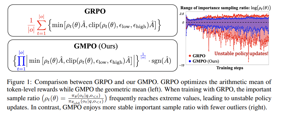
7) Geometric Mean Policy Optimization (GMPO)

GMPO (Geometric-Mean Policy Optimization) is a very “surgical” fix to a very specific GRPO failure mode: token-level importance ratios $\rho_{i,t}$ can develop nasty outliers, and GRPO’s arithmetic-mean objective is too sensitive to those outliers, so one or two extreme tokens can dominate the update and push the policy into unstable territory. The GMPO paper visualizes this directly: during GRPO training the range of $\log \rho_t(\theta)$ keeps expanding with lots of extreme spikes (“unstable policy updates”), while GMPO keeps the ratio range tighter with fewer outliers.

GMPO

In GRPO, each generated token contributes an importance-weighted term using:

$$\rho_{i,t}(\theta)=\frac{\pi_\theta(o_{i,t}\mid q,o_{i,<t})}{\pi_{\theta_{\text{old}}}(o_{i,t}\mid q,o_{i,<t})}$$

If $\rho_{i,t}$ gets extreme (very large or very small), the corresponding token’s contribution to the update can become extreme too. The GMPO paper’s diagnosis is: GRPO optimizes an arithmetic mean over token-level “rewards” (importance-weighted advantages), and the arithmetic mean is notoriously sensitive to outliers, so a few pathological tokens can drive aggressive updates, which then create even more extreme $\rho$’s, and the loop feeds itself.

Conceptually:

GRPO: average token contributions with an arithmetic mean: $\frac{1}{|o_i|}\sum_t (\cdot)$
GMPO: aggregate token contributions with a geometric mean: $\left(\prod_t (\cdot)\right)^{1/|o_i|}$

Geometric mean is much more robust: one extreme token can’t blow up the whole objective as easily because products + root behave like averaging in log-space.

The paper first introduces GMPO (ignoring clipping for the moment) as maximizing the geometric mean of token-level terms; they also include a $\mathrm{sgn}(\hat A_i)$ so the optimization direction stays correct when the group advantage is negative:

$$ \mathcal{J} ^ { * } _ { \text{GMPO} } ( \pi _ \theta ) = \mathbb{E} _ { q \sim \mathcal{Q} , { o _ i } _ { i = 1 } ^ G \sim \pi _ { \theta _ { \text{old} } } ( \cdot | q ) } $$

$$ \left[ \frac{1}{G} \sum _ { i = 1 } ^ G \left( \prod _ { t = 1 } ^ { | o _ i | } | \rho _ { i,t } ( \theta ) \hat{A} _ i | \right) ^ { \frac{1}{ | o _ i | } } \cdot \text{sgn} ( \hat{A} _ i ) \right] $$

Then they “expand” it to include PPO-style clipping at the token level:

$$\mathcal{J} _ { \text{GMPO} } ( \pi _ \theta ) = \mathbb{E} _ { q , { o _ i } } [ \text{Group Average of Response Scores} ]$$

Step 1: Per-Token Clipped Signal $$\mathcal{C} _ { i,t } = \min [ \rho _ { i,t } ( \theta ) \hat{A} _ i , \text{clip} ( \rho _ { i,t } ( \theta ) , \epsilon _ { \text{low} } , \epsilon _ { \text{high} } ) \hat{A} _ i ]$$

Step 2: Sequence Geometric Mean $$\text{Score} _ i = ( \prod _ { t = 1 } ^ { | o _ i | } | \mathcal{C} _ { i,t } | ) ^ { 1 / | o _ i | } \cdot \text{sgn} ( \hat{A} _ i )$$

Step 3: Final Objective $$\mathcal{J} = \frac{1}{G} \sum _ { i = 1 } ^ G \text{Score} _ i$$

The paper shows: $$| \mathcal{J} ^ { * } _ { \text{GMPO} } | \le | \mathcal{J} ^ { * } _ { \text{GRPO} } |$$ using the classic AM–GM inequality intuition: geometric mean is always $\le$ arithmetic mean for non-negative numbers. That “narrower range” is their theoretical proxy for lower variance / less sensitivity to outliers → more stable updates.

$$ \left| \mathcal{J} ^ { * } _ { \text{GMPO} } ( \pi _ \theta ) \right| = \mathbb{E} _ { q \sim \mathcal{Q} , { o _ i } _ { i = 1 } ^ G \sim \pi _ { \theta _ { \text{old} } } ( \cdot | q ) } \left[ \frac{1}{G} \sum _ { i = 1 } ^ G \left( \prod _ { t = 1 } ^ { | o _ i | } | \rho _ { i,t } ( \theta ) \hat{A} _ i | \right) ^ { \frac{1}{ | o _ i | } } \right] $$

$$ \le \mathbb{E} _ { q \sim \mathcal{Q} , { o _ i } _ { i = 1 } ^ G \sim \pi _ { \theta _ { \text{old} } } ( \cdot | q ) } \left[ \frac{1}{G} \sum _ { i = 1 } ^ G \frac{1}{ | o _ i | } \sum _ { t = 1 } ^ { | o _ i | } | \rho _ { i,t } ( \theta ) \hat{A} _ i | \right] = \left| \mathcal{J} ^ { * } _ { \text{GRPO} } ( \pi _ \theta ) \right| $$

Gradient intuition:

This is the most important “mechanistic” difference.

GRPO gradient: token $t$ is weighted by its own ratio $\rho_{i,t}$. One extreme token can blow up its gradient weight.
GMPO gradient: token $t$ is weighted by the geometric mean of ratios across the whole sequence, roughly $\left(\prod_k \rho_{i,k}\right)^{1/|o_i|}$. So even if one $\rho_{i,t}$ is extreme, the sequence-level geometric mean damps it.

$$ \nabla _ { \theta } \mathcal{J} ^ { * } _ { \text{GRPO} } ( \pi _ \theta ) | _ { q , o _ i } = \frac{1}{ G \cdot | o _ i | } \sum _ { t = 1 } ^ { | o _ i | } {\color{red}\rho _ { i,t } ( \theta )} \cdot \hat{A} _ i \cdot \nabla _ { \theta } \log \pi _ \theta ( o _ { i,t } | q , o _ { i, <t } ) $$

$$ \nabla _ { \theta } \mathcal{J} ^ { * } _ { \text{GMPO} } ( \pi _ \theta ) | _ { q , o _ i } = \frac{1}{ G \cdot | o _ i | } \sum _ { t = 1 } ^ { | o _ i | } \left ( \prod _ { k = 1 } ^ { | o _ i | } {\color{blue}\rho _ { i,k } ( \theta )} \right) ^ { \frac{1}{ | o _ i | } } \cdot \hat{A} _ i \cdot \nabla _ { \theta } \log \pi _ \theta ( o _ { i,t } | q , o _ { i, <t } ) $$

(i) Token-level clipping (vs sequence-level clipping)

The paper argues sequence-level clipping is too aggressive: if you clip the whole product term at once, once the clip triggers you can zero out gradients for all tokens in the sequence, throwing away useful learning signal. Token-level clipping is more “local” and tends to be more stable.

(ii) Clip wider (in the DAPO spirit, but safer)

Like DAPO, they want more exploration by widening the clip range (because tight clipping can make policies go deterministic early). But they claim GMPO can afford wider clipping without exploding, because the geometric mean suppresses outliers in $\rho$ more naturally.

8) Router-Shift Policy Optimization (RSPO)

RSPO sits in a very specific corner of post-training: off-policy RL (multiple update rounds per batch) for MoEs. In dense LMs, “off-policy drift” is mostly about the token distribution $\pi_\theta(\cdot)$ moving away from the behavior policy $\pi_{\theta_{\text{old}}}$. In MoE, you implicitly introduce a second stochastic system: the router distribution over experts. After an update, the router can (a) change the top-K experts selected for the same token, and/or (b) keep the same top-K but reweight them. The paper emphasizes both effects, and notes that even modest changes in routing can cause large fluctuations in token-level importance ratios, frequently triggering clipping and injecting extra variance.

GRPO’s token-level IS ratios and clipping were designed for settings where the policy is a single distribution over actions. In MoE, the induced distribution over tokens is a mixture whose components and mixing weights can change abruptly between updates.

GRPO in MoE exhibits two coupled sources of instability:

(1) Router-induced IS volatility (routing fluctuations)

Let the token probability decompose as a mixture:

$\pi_\theta(o_{t}\mid h_t)=\sum_{e\in\mathcal{E}} r_\phi(e\mid h_t),\pi_{\theta,e}(o_t\mid h_t)$

where $r_\phi$ is the router distribution (parameters $\phi$), and $\pi_{\theta,e}$,is the expert-conditional distribution.

The token-level importance ratio used by GRPO is: $$ w_t(\theta)=\frac{\pi_\theta(o_t\mid h_t)}{\pi_{\theta_{\text{old}}}(o_t\mid h_t)} $$

Even if the expert networks $\pi_{\theta,e}$ barely changed, a change in $r_\phi(e\mid h_t)$ can shift $\pi_\theta(o_t\mid h_t)$ sharply, especially when mass moves between a few high-weight experts. This pushes $w_t$ into the clip region more often (or creates outliers that dominate gradients before clipping), which is exactly the failure mode they illustrate and connect to prior MoE observations (e.g., StableMoE).

(2) Variance mismatch (sequence reward vs token IS)

Most RLVR setups attach reward at the sequence level (rule-based verifier / outcome reward), then propagate learning through token-level policy gradients. GRPO often combines sequence-level advantage with token-level IS weights, which is already a mismatch in dense LMs; in MoE it’s amplified because variance at the token level now includes router variance. The RSPO paper flags this explicitly as “variance mismatch” that, together with routing fluctuations, hinders stable learning.

RSPO objective: geometric-mean aggregation + token-level clipping + router-shift reweighting

RSPO keeps a sequence-level aggregation (geometric mean over tokens), but uses token-level clipping (to avoid “all-or-nothing” pruning), and multiplies each token’s contribution by a router-shift ratio $\gamma_{i,t}$ that down-weights tokens whose routing changed too much.

$$ \text{Sequence Score} _ i = [ \prod _ { t = 1 } ^ { | o _ i | } ( \mathcal{W} _ { i,t } \cdot \gamma _ { i,t } ) ] ^ { \frac{ \text{sgn} ( \hat{A} _ i ) }{ | o _ i | } } $$

$$ \mathcal{W} _ { i,t } = \min [ ( w _ { i,t } ( \theta ) ) ^ { \text{sgn} ( \hat{A} _ i ) } , \text{clip} ( ( w _ { i,t } ( \theta ) ) ^ { \text{sgn} ( \hat{A} _ i ) } , \varepsilon _ 1 , \varepsilon _ 2 ) ] $$

$$ \mathcal{J} _ { \text{RSPO} } ( \pi _ \theta ) = \mathbb{E} _ { x \sim \mathcal{Q} , { o _ i } _ { i = 1 } ^ G \sim \pi _ { \text{old} } } \left[ \frac{1}{G} \sum _ { i = 1 } ^ G \mathcal{S} _ i \cdot \hat{A} _ i \right] $$

$w_{i,t}(\theta)$: token-level importance sampling ratio (same as GRPO), comparing current vs old policy for token $o_{i,t}$:
$\hat A_i$: (group) advantage for the $i$-th response $o_i$, defined as in GRPO (sequence-level signal used to scale updates).
$\mathrm{sgn}(\hat A_i)$: sign of the advantage (+1 if $\hat A_i>0$, −1 if $\hat A_i<0$); used so clipping behaves correctly for positive vs negative updates:
$γ_{i,t}$: router shift ratio for token $t$ in response $o_i$; measures routing drift between old and current routers and scales (down-weights) the token’s contribution after clipping.
$r^{(\ell)}_{\phi}(\cdot)$: routing score / routing probability under router parameters $\phi$ at MoE layer $\ell$.
$r^{(\ell)}_{\phi _ {\text{old}}}(\cdot)$: the same, but for the old router $\phi_{\text{old}}$.
$e^{(\ell)}_{i,t}$: the expert associated with token position $(i,t)$ at layer $\ell$ (often top-K experts are considered).
Top-K experts: RSPO estimates routing drift by averaging routing-score differences over the top-K experts that were activated under the old policy during log-prob computation.
Multiplicative aggregation across layers: since routing deviations can accumulate with depth, per-layer router shifts are combined multiplicatively to form the final $\gamma_{i,t}$ (implemented via sums of log differences inside an $\exp(\cdot)$.
Where $\gamma_{i,t}$ is applied: $\gamma_{i,t}$ is used as a reweighting factor after token-level clipping, preserving the original trust-region behavior while further damping tokens with excessive routing drift.
the router-shift weight $\gamma_{i,t}$:

$$ \gamma _ { i,t } = \exp \left( - \frac{1}{ L } \sum _ { \ell = 1 } ^ { L } \frac{1}{ K } \sum _ { k = 1 } ^ { K } | \log r _ \phi ^ { ( \ell ) } ( e _ { i,t } ^ { ( \ell,k ) } | x, y _ { i,<t } ) - \log r _ { \phi _ { \text{old} } } ^ { ( \ell ) } ( e _ { i,t } ^ { ( \ell,k ) } | x, y _ { i,<t } ) | \right) $$

$\gamma_{i,t}=\max(\gamma_{i,t},\gamma_{\min})$ $\text{Use } \mathrm{sg}[\gamma_{i,t}] \text{ (stop-gradient) so } \gamma_{i,t} \text{ acts only as a sample weight.}$

What $\gamma_{i,t}$ is measuring?

For each generated token position $t$ in response $i$, RSPO looks across:

all MoE layers $\ell = 1,\dots,L$
the top-K experts considered/activated at that layer, indexed by $k=1,\dots,K$

and compares the router’s log routing scores under the current router $\phi$ vs the old router $\phi_{\text{old}}$: $$ \log r _ \phi ^ { ( \ell ) } ( e _ { i,t } ^ { ( \ell,k ) } | x, y _ { i,<t } ) \quad \text{vs} \quad \log r _ { \phi _ { \text{old} } } ^ { ( \ell ) } ( e _ { i,t } ^ { ( \ell,k ) } | x, y _ { i,<t } ) $$ It takes an absolute difference $|\cdot|$ (so “changed up or down” both count), averages over experts and layers $\frac{1}{L}\sum_{\ell}\frac{1}{K}\sum_k$, then exponentiates the negative of that: $$\gamma_{i,t}=\exp(-\text{avg drift})$$

Why the exponential form?

If the router barely changed: average drift $\approx 0$ → $\gamma_{i,t}\approx e^0=1$.
If the router changed a lot: average drift large → $\gamma_{i,t}$ becomes small (close to 0).

So $\gamma_{i,t}\in(0,1]$ acts like a soft reliability score:

$\gamma_{i,t}\approx 1$: routing is consistent → token-level IS ratios are more trustworthy.
$\gamma_{i,t}\ll 1$: routing drift is big → token-level IS ratios are noisy/unreliable → down-weight this token’s contribution.

$γ_{i,t}$ is a routing-drift penalty: the more the router changed for token $t$, the less RSPO lets that token push the policy update

Why “stop-gradient” through $\gamma_{i,t}$?

Gradients do not flow into the router via $\gamma$. Otherwise, the optimizer could “cheat” by manipulating routing just to inflate $\gamma$, or you’d introduce messy second-order interactions where $\gamma$ itself becomes a learnable pathway. With stop-grad, $\gamma$ is purely a stability filter: it modulates how much you trust the token’s update, but doesn’t become a new optimization target.

9) Soft Adaptive Policy Optimization (SAPO)

Group-based RL for LLM post-training typically relies on importance ratios to reuse trajectories across policy updates, but in practice those ratios are noisy at the token level, and the variance is especially acute in Mixture-of-Experts models, where routing heterogeneity and long generations amplify per-token deviations. The standard remedy in GRPO is hard token clipping: once a token’s ratio exits a fixed band, its contribution is effectively truncated to zero gradient, which stabilizes extreme steps but creates a brittle trade-off, tight clipping wastes samples and kills learning signal, while looser clipping admits off-policy noise and destabilizes optimization. GSPO shifts the trust region to the sequence level to enforce coherence with sequence rewards, but this introduces a different pathology: a small number of outlier tokens can push the sequence ratio beyond the clip band, causing the entire sequence’s gradients (including many near-on-policy, informative tokens) to be suppressed. Soft Adaptive Policy Optimization (SAPO) is proposed to resolve this “hard-gate brittleness” by replacing clipping with a temperature-controlled soft gate over importance ratios: near the on-policy point ($r\approx 1$), gradients are preserved to encourage learning and exploration; as ratios drift, updates are attenuated smoothly rather than truncated, retaining useful signal from moderate deviations while damping high-variance outliers. Crucially, SAPO is designed to be sequence-coherent yet token-adaptive: under empirically common conditions (small policy steps and low intra-sequence dispersion of token log-ratios), the average token gate concentrates into a smooth sequence-level gate (GSPO-like behavior, but with a continuous trust region), while in the presence of heterogeneous or outlier tokens it selectively down-weights only the offending tokens instead of collapsing the whole sequence.

SAPO objective: “grouped RL” + a gating function over importance ratios:

SAPO optimizes a grouped surrogate:

$$ \mathcal{J} ( \theta ) = \mathbb{E} _ { q \sim \mathcal{D} , { y _ i } _ { i = 1 } ^ G \sim \pi _ { \theta _ { \text{old} } } ( \cdot | q ) } $$

$$ \left[ \frac{1}{G} \sum _ { i = 1 } ^ G \frac{1}{ | y _ i | } \sum _ { t = 1 } ^ { | y _ i | } f _ { i,t } ( r _ { i,t } ( \theta ) ) \hat{A} _ { i,t } \right] $$

$q\sim \mathcal D$: prompt/query drawn from your prompt distribution.
${y_i}_{i=1}^G \sim \pi _ {\theta _ {\text{old}}}(\cdot|q)$: you sample a group of $G$ responses from the behavior policy (the “old” policy). This is the GRPO/GSPO regime: generate many candidates, compare within a group, update current policy.
$\frac{1}{|y_i|}\sum_t$: length-normalization so long generations don’t dominate purely by having more tokens.
$\hat A_{i,t}$: advantage signal (often group-normalized reward); in many group-RL setups it’s constant across tokens in a response, i.e.$\hat A_{i,t}=\hat A_i$. It tells you “this whole sampled trajectory was better/worse than its siblings.”
$r_{i,t}(\theta)$: token-level importance ratio:

$$ r_{i,t}(\theta)=\frac{\pi_\theta(y_{i,t}\mid q,y_{i,<t})}{\pi_{\theta_{\text{old}}}(y_{i,t}\mid q,y_{i,<t})} $$

If $r\approx 1$: current policy is close to behavior policy at that token (near on-policy). If $r$ is far from 1, you’re reusing a token that is effectively off-policy for the current model, high-variance / risky to trust.

The entire novelty is the choice of the gating function $f_{i,t}(\cdot)$: instead of GRPO/GSPO’s hard clipping, SAPO uses a smooth, temperature-controlled soft gate that attenuates off-policy tokens rather than truncating them.

The SAPO gate:

$$ f _ { i,t } ( x ) = \sigma ( \tau _ { i,t } ( x - 1 ) ) \cdot \frac{ 4 }{ \tau _ { i,t } } $$

Where the temperature parameter $\tau _ { i,t }$ is:

$$ \tau _ { i,t } = \tau _ { \text{pos} } \quad \text{if} \quad \hat{A} _ { i,t } > 0 \quad \text{else} \quad \tau _ { \text{neg} } $$

Centering at $x−1$: the “trust region center” is $r=1$ (on-policy). Everything is about how far your current policy deviates from the behavior policy.
$\sigma(\tau(x-1))$: smooth monotone gate. Temperature $\tau$ controls steepness:
- small $\tau$ ⇒ gentle decay (more tolerant of deviation),
- large $\tau$ ⇒ sharp decay (more conservative).
Asymmetric temperatures $\tau_{\text{pos}}$, $\tau_{\text{neg}}$: SAPO intentionally treats positive-advantage and negative-advantage updates differently.
The factor $4/\tau$ looks like a hack, but it’s actually a calibration: it makes the resulting gradient weight nicely normalized so that the effective weight peaks at 1 at the on-policy point. This is why SAPO preserves “unclipped behavior” near $r=1$ regardless of $\tau$.

Differentiating SAPO gives a weighted log-policy gradient:

if we differentiate the SAPO objective using $\nabla_\theta r = r\nabla_\theta \log \pi_\theta(\cdot)$ we get:

$$ \nabla _ \theta \mathcal{J} ( \theta ) = \mathbb{E} \left[ \frac{1}{ G } \sum _ { i = 1 } ^ G \frac{1}{ | y _ i | } \sum _ { t = 1 } ^ { | y _ i | } w _ { i,t } ( \theta ) \cdot r _ { i,t } ( \theta ) \cdot \nabla _ \theta \log \pi _ \theta ( y _ { i,t } | q , y _ { i, <t } ) \cdot \hat{A} _ { i,t } \right] $$

where - $$ w_{i,t}(\theta)=4 \ p_{i,t}(\theta)\big(1-p_{i,t}(\theta)\big), \qquad p_{i,t}(\theta)=\sigma\big(\tau_{i,t}(r_{i,t}(\theta)-1)\big). $$

$w_{i,t}$ is a smooth trust-region kernel

$p(1−p)$ is maximized at $p =1/2$.
$p=1/2$ happens exactly when $\tau(r-1)=0$ ⇒ $r=1$.
Therefore, $w_{i,t}$ peaks at 1 when $r_{i,t}=1$ and decays smoothly as $r$ moves away from 1.

Concretely:

If $r\approx 1$ : $w\approx 1$, SAPO behaves like the unclipped objective (strong learning signal).
If $r$ is moderately off: $w\in(0,1)$, you still learn but cautiously.
If $r$ is extremely off: $w\to 0$, SAPO essentially ignores those tokens, but without a discontinuous cliff (unlike hard clipping).

This is why the paper calls SAPO a continuous trust region: the “trust” shrinks continuously as deviation grows, rather than flipping from 1 to 0 at a fixed $\epsilon$.

Why SAPO uses two different temperatures $\tau_{\text{pos}}$ and $\tau_{\text{neg}}$?

Negative-advantage token updates are intrinsically more destabilizing in large-vocabulary softmax policies, because their gradients spread across many logits (many “unsampled” tokens). So SAPO makes negative-token gates decay faster by setting $\tau_{\text{neg}}>\tau_{\text{pos}}$.

Mathematical Intuition:

Let the model output logits $z \in \mathbb{R}^{|V|}$ at a decoding step $t$, where $z_v$ is the logit for vocabulary token $v$. The policy is a softmax:

$$ \pi _ \theta(v \mid q, y _ {<t}) = \frac{e^{z _ v}}{\sum _ {v’\in V} e^{z _ v’}}. $$

A sampled token at this step is $y_t$ (the action taken). In policy-gradient RL, you weight the log-prob gradient by an advantage $\hat A_t$ (or $\hat A_i$ shared across tokens in a sequence):

$$ \text{token contribution} \propto \hat A_t , \nabla_\theta \log \pi_\theta(y_t \mid q,y_{<t}). $$

We want $\frac{\partial}{\partial z_v} \big(\hat A_t \log \pi_\theta(y_t)\big)$.

First recall the standard softmax-log derivative:

$$ \frac{\partial \log \pi _ \theta(y _ t)}{\partial z _ v} = \mathbf{1}[v = y _ t] - \pi _ \theta(v). $$

Multiply by $\hat A_t$:

$$ \frac{\partial \log \pi _ \theta\left(y _ {i,t}\mid q, y _ {i,<t}\right),\hat A _ {i,t}}{\partial z _ v} = \frac{\partial \pi _ \theta\left(y _ {i,t}\mid q, y _ {i,<t}\right)}{\partial z _ v}\cdot \frac{\hat A _ {i,t}}{\pi _ \theta\left(y _ {i,t}\mid q, y _ {i,<t}\right)} $$

$$ = \frac{ \mathbf{1}( v = y _ { i,t } ) \cdot e ^ { z _ { y _ { i,t } } } \sum _ { v’ \in V } e ^ { z _ { v’ } } - e ^ { z _ { y _ { i,t } } } \cdot e ^ { z _ v } }{ ( \sum _ { v’ \in V } e ^ { z _ { v’ } } ) ^ 2 } \cdot \frac{ \hat{A} _ { i,t } }{ \pi _ \theta ( y _ { i,t } | q, y _ { i,<t } ) } $$

For the Sampled Token ($v = y _ { i,t }$): $$ \text{Gradient} = ( 1 - \pi _ \theta ( y _ { i,t } | q , y _ { i,<t } ) ) \cdot \hat{A} _ { i,t } $$
For All Other Tokens ($v \neq y _ { i,t }$): $$ \text{Gradient} = - \pi _ \theta ( v | q , y _ { i,<t } ) \cdot \hat{A} _ { i,t } $$

$\mathbf{1}[v=y_t]$: indicator for the sampled token.
$\pi_\theta(v)$: model’s probability mass on token $v$ at this state.
$\hat A_t$: advantage; sign determines whether to reinforce or suppress the sampled action.

Intuition: positive vs. negative advantages change the direction of mass movement

Case A: $\hat A_t > 0$ (positive advantage)

For the sampled token $v=y_t$: $$ \Delta z_{y_t} \propto (1-\pi_\theta(y_t)),\hat A_t > 0 $$ So we increase the sampled token’s logit (make it more likely).

For every other token $v\neq y_t$: $$ \Delta z_v \propto -\pi_\theta(v)\hat A_t < 0 $$ So we decrease all other logits slightly.

Net effect: probability mass flows toward the sampled token.

Case B: $\hat A_t < 0$ (negative advantage)

Now signs flip.

For the sampled token:

$$ \Delta z_{y_t} \propto (1-\pi_\theta(y_t))\hat A_t < 0 $$

So we decrease the sampled token’s logit (make it less likely).

For every other token: $$ \Delta z_v \propto -\pi_\theta(v)\hat A_t > 0 $$

So we increase logits of all other tokens.

Net effect: probability mass is pushed away from the sampled token and spread across the rest of the vocabulary.

Why negative updates are more destabilizing in LLMs?

In LLM RL, the action space is the vocabulary: $|V|$ is huge (often $10^5–10^6$). At a given state, only a small subset of tokens are “reasonable.” The paper’s point is:

With negative advantage, you are increasing logits for an enormous set of “unsampled” tokens.
Even though each individual increase is scaled by $\pi_\theta(v)$, there are so many $v\neq y_t$ that the update can “diffuse” into lots of irrelevant directions.
This diffusion is especially harmful off-policy (importance ratios far from 1), where variance is already high.

You can see this from the total “push” to unsampled logits:

$$ \sum_{v\neq y_t} \Delta z_v \propto \sum_{v\neq y_t} \big(-\pi_\theta(v)\hat A_t\big) = -(1-\pi_\theta(y_t))\hat A_t. $$

So the aggregate magnitude is comparable to the sampled-token magnitude, but it’s distributed over $|V|-1$ coordinates, i.e., a very high-dimensional “spray.” For $\hat A_t<0$, that spray points in a direction that can introduce instability (lots of tiny increases to many logits can change the distribution in unintuitive ways, especially under large steps / off-policy noise).

How SAPO uses temperature to tame this: $\tau_{\text{neg}} > \tau_{\text{pos}}$

SAPO’s token gate uses a temperature $\tau$ that controls how fast gradients decay as the importance ratio $r_{t}$ deviates from 1. The effective weight is a smooth kernel that peaks at $r=1$ and shrinks as $|r-1|$ grows:

$$ w(r) = 4\sigma(\tau(r-1))\big(1-\sigma(\tau(r-1))\big) = \mathrm{sech}^2\left(\frac{\tau}{2}(r-1)\right). $$

Larger $\tau$ ⇒ faster decay of $w(r)$ away from $r=1$ (more aggressive damping of off-policy tokens).
SAPO sets:

Positive Advantage ($\hat{A} _ t > 0$): $$ \tau = \tau _ { \text{pos} } $$
Negative Advantage ($\hat{A} _ t \le 0$): $$ \tau = \tau _ { \text{neg} } $$

Constraint: $$ \tau _ { \text{neg} } > \tau _ { \text{pos} } $$

So when $\hat A_t<0$, the update is the “spray to unsampled logits” case, and SAPO attenuates it more strongly as soon as it becomes off-policy, reducing variance and early collapse risk.

SAPO/GRPO/GSPO can be written as a single gated surrogate (unified-surrogate) where the only difference is the gating function $f_{i,t}$:

$$ \mathcal{J}(\theta) =\mathbb{E}\Bigg[\frac{1}{G}\sum_{i=1}^G \frac{1}{|y_i|}\sum_{t=1}^{|y_i|} f_{i,t}\big(r_{i,t}(\theta)\big)\hat A_{i,t}\Bigg], \qquad r_{i,t}(\theta)=\frac{\pi_\theta(y_{i,t}\mid q,y_{i,<t})}{\pi_{\theta_{\text{old}}}(y_{i,t}\mid q,y_{i,<t})}. $$

where, $f_{i,t}(·)$ is an algorithm-specific gating function.

GSPO is “sequence-level” because it replaces token ratios by the length-normalized sequence ratio (geometric mean):

$$ s_i(\theta) =\left(\frac{\pi_\theta(y_i\mid q)}{\pi_{\theta_{\text{old}}}(y_i\mid q)}\right)^{1/|y_i|} =\exp\left(\frac{1}{|y_i|}\sum_{t=1}^{|y_i|}\log r_{i,t}(\theta)\right), $$

and then gates using $s_i(\theta)$ (token-invariant within a sequence), while GRPO gates each token via hard clipping of $r_{i,t}$. SAPO instead uses a soft gate:

$$ f^{\text{SAPO}} _ {i,t}(r)=\frac{4}{\tau _ i}\sigma\big(\tau _ i(r-1)\big),\qquad \tau _ i=\tau _ {\text{pos}}\ \text{if }\hat A _ i>0,\ \text{else }\tau _ {\text{neg}}, $$

so its gradient contribution is smoothly down-weighted as $r$ moves away from the on-policy point $r=1$, rather than being abruptly zeroed by a hard clip.

Algorithm-specific $f _ {i,t}$.

The algorithms differ in the choice of $f _ {i,t}$:

$$ \textbf{SAPO:}\quad f^{\mathrm{SAPO}} _ {i,t}\big(r _ {i,t}(\theta)\big) = \frac{4}{\tau _ i}\sigma\big(\tau _ i,(r _ {i,t}(\theta)-1)\big), \qquad \tau _ i= \begin{cases} \tau _ {\text{pos}}: & \hat A _ i>0,\ \tau _ {\text{neg}}: & \hat A _ i\le 0. \end{cases} $$

$$ \textbf{GRPO:}\quad f^{\mathrm{GRPO}} _ {i,t}\big(r _ {i,t}(\theta);\hat A _ i\big) = \begin{cases} \min\big(r _ {i,t}(\theta),1+\epsilon\big): & \hat A _ i>0,\ \max\big(r _ {i,t}(\theta),1-\epsilon\big): & \hat A _ i\le 0. \end{cases} $$

$$ \textbf{GSPO:}\quad f^{\mathrm{GSPO}} _ {i,t}\big(r _ {i,t}(\theta);\hat A _ i\big) = f^{\mathrm{seq}} _ {i,t}\big(s _ i(\theta);\hat A _ i\big) = \begin{cases} \min\big(s _ i(\theta),1+\epsilon\big): & \hat A _ i>0,\ \max\big(s _ i(\theta),1-\epsilon\big): & \hat A _ i\le 0. \end{cases} $$

GSPO’s $f_{i,t}$ is token-invariant within a sequence, while SAPO and GRPO are token-dependent.

Differentiating the unified surrogate gives the common “gate × ratio × logprob-grad × advantage” form: $$ \nabla _ \theta \mathcal{J}(\theta) =\mathbb{E}\Bigg[\frac{1}{G}\sum _ {i=1}^G \frac{1}{|y _ i|}\sum _ {t=1}^{|y _ i|} f’ _ {i,t}\big(r _ {i,t}(\theta)\big)\ r _ {i,t}(\theta)\ \nabla _ \theta\log\pi _ \theta(y _ {i,t}\mid q,y _ {i,<t})\hat A _ {i,t}\Bigg]. $$

For SAPO specifically, using $\sigma(x)(1-\sigma(x))=\tfrac14\mathrm{sech}^2(x/2)$:

$$ f _ {i,t}^{\mathrm{SAPO}'}\big(r _ {i,t}(\theta)\big) = 4\sigma\big(\tau _ i(r _ {i,t}(\theta)-1)\big)\Big(1-\sigma\big(\tau _ i(r _ {i,t}(\theta)-1)\big)\Big) = \mathrm{sech}^2\left(\frac{\tau _ i}{2}\big(r _ {i,t}(\theta)-1\big)\right). $$

The post-training landscape is clearly past the era of “just use PPO.” What GRPO and its descendants have exposed is a deeper pattern: most of the practical wins come from how we control trust and variance in the update, where the trust region lives (token vs. sequence), how sharply we enforce it (hard clip vs. soft gate), and how we keep exploration alive without letting off-policy noise and long-horizon credit assignment blow up the run. The “algorithm” is increasingly a choice of gating function, normalization scheme, and stability knobs tailored to the geometry of language modeling, huge vocabularies, long sequences, and a reward signal that’s sparse, delayed, and often noisy.

If there’s one takeaway to carry forward, it’s that the next wave of progress will come less from inventing yet another acronym and more from making these design axes explicit and measurable. As you experiment, treat these methods as a toolkit: pick the gate that matches your reward structure, pick the unit of coherence that matches your objective (token-local vs. sequence-global), and tune conservativeness in a way you can defend with plots. The exciting part is that we’re still early: as verifiable rewards, multimodal policies, and long-context training become standard, these “small” choices about clipping, gating, and variance control are going to be the difference between models that merely improve and systems that train reliably at scale.

1) From PPO to GRPO#

2) GRPO: Group Relative Policy Optimization (GRPO)#

Key changes vs PPO#

3) DR.GRPO (GRPO done Right)#

4) GSPO (Group Sequence Policy Optimization)#

5) Decoupled Clip and Dynamic Sampling Policy Optimization (DAPO)#

6) CISPO (Clipped IS-weight Policy Optimization)#

7) Geometric Mean Policy Optimization (GMPO)#

8) Router-Shift Policy Optimization (RSPO)#

9) Soft Adaptive Policy Optimization (SAPO)#

References#