Transformer models have become the backbone of modern AI, yet their remarkable performance still comes with a critical limitation: we lack a clear understanding of how information is processed inside them. Traditional evaluation focuses on outputs, but this leaves open the deeper question of what actually happens between layers as a model learns to reason. In our work, we approach this problem through a geometric lens, using Optimal Transport to measure how entire distributions of representations shift across layers. This perspective allows us to contrast trained and untrained models, revealing that training does not simply tune parameters, but organizes computation into a structured three-phase strategy: encoding, refinement, and decoding, underpinned by an information bottleneck. By making this internal structure visible, we aim to move closer to principled interpretability, where understanding a model means understanding the pathways of information it discovers through learning.
Bridging Information Theory and Representation Geometry
One of the most influential perspectives for understanding deep neural networks (DNNs) comes from information theory, pioneered by Professor Naftali Tishby and collaborators. Instead of treating neural networks as inscrutable black boxes, this framework casts them as information processing systems. The central idea is simple but powerful: learning in a DNN is not just about memorizing patterns; it is about shaping how information flows, compresses, and refines across layers.
At its core, a neural network can be viewed as a Markov chain: $$
X \rightarrow h_1 \rightarrow h_2 \rightarrow \cdots \rightarrow h_m \rightarrow \hat{Y}
$$
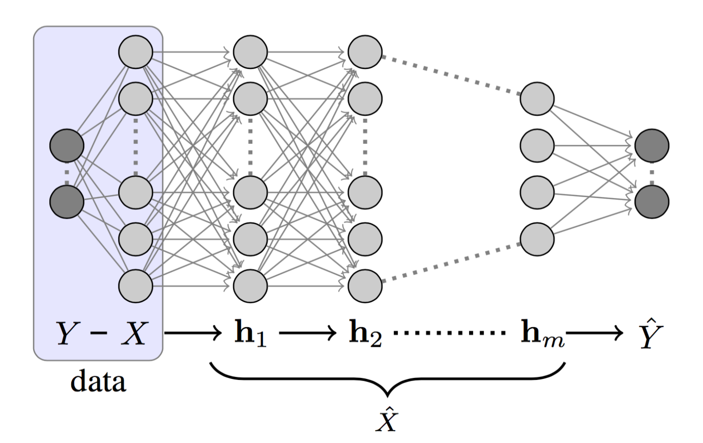
Each layer depends only on the previous one. This structure has important consequences. By the Data Processing Inequality (DPI), mutual information, the measure of how much one variable tells us about another, can only decrease as we move forward through the chain. In practice, this means that as raw input passes through successive layers, the network must compress away irrelevant details while retaining what matters for predicting Y.
This intuition is formalized in the Information Bottleneck (IB) principle. The goal of a hidden representation is twofold:
- Preserve as much relevant information about the target as possible: $I(\hat{X};Y)$
- Discard irrelevant information from the input: $I(X; \hat{X})$
The IB framework describes this as an optimization problem: find the “sweet spot” where representations are maximally compressed yet maximally predictive. In other words, the network learns to forget just enough of the input to generalize well, while keeping what is essential for the task.
To visualize this process, Tishby introduced the information plane, where each hidden layer is plotted based on two values: mutual information with the input: $I(X; T_i)$ and with the output: $I(T_i; Y)$. During training, layers trace characteristic trajectories across this plane. Early on, they rapidly climb upwards, capturing more information about the target (the fitting phase). Later, they drift leftwards, compressing redundant details from the input (the compression phase). This two-stage dynamic suggests that generalization in deep learning is inseparable from information compression.
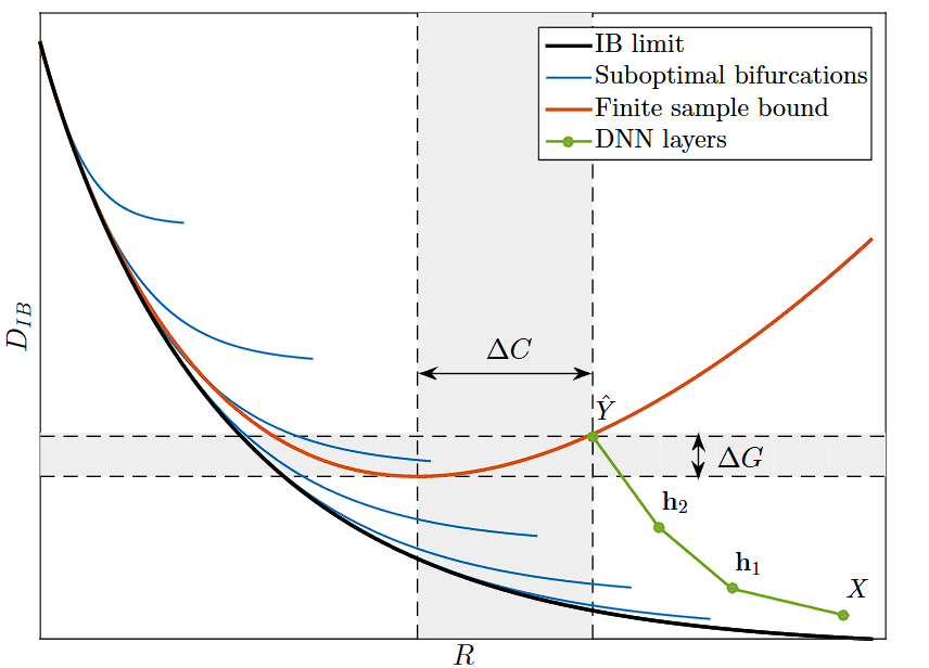
Beyond interpretation, the IB framework also provides new theoretical insights. Traditional complexity bounds (e.g., VC dimension) fail to explain why massive over-parameterized models can generalize so well. But by framing generalization error in terms of mutual information, the IB view shows that compression directly improves generalization, each bit of discarded input information effectively multiplies the sample efficiency.
Limitations
While the IB theory is an elegant explanation for learning, its primary challenge has been empirical validation. The theory relies on measuring mutual information $I(X; T_i)$ and $I(T_i; Y)$, which is notoriously difficult to calculate accurately for high-dimensional, continuous data like neural network activations. This has led to debates about whether the observed “compression phase” is a genuine phenomenon or an artifact of the measurement technique, especially in modern networks that use ReLU activations.
How Optimal Transport Provides a Solution?
The starting point for this research was a question that has long fascinated us: what does it really mean for a neural network to “learn” internally? Information theory, particularly the Information Bottleneck (IB) framework pioneered by Naftali Tishby, gave us our first conceptual lens. It suggested that learning is a process of compressing input representations while preserving task-relevant information, effectively building an efficient “information highway” from inputs to outputs. The idea that networks undergo phases of fitting and compression, visible on the information plane, framed our thinking: learning is not just parameter tuning, but a reorganization of information flow.
At the same time, we were intrigued by another mathematical tradition: Optimal Transport (OT). Originally formulated by Gaspard Monge in the 18th century and later relaxed by Leonid Kantorovich, OT asks: what is the most efficient way to move mass from one distribution to another? This perspective felt deeply aligned with our information-theoretic intuitions. If layer activations in a neural network can be seen as empirical distributions, then the transformation from one layer to the next is nothing more than a transport problem. The “cost” of moving one distribution into another could give us a direct, geometric measure of how much work the network performs between layers.
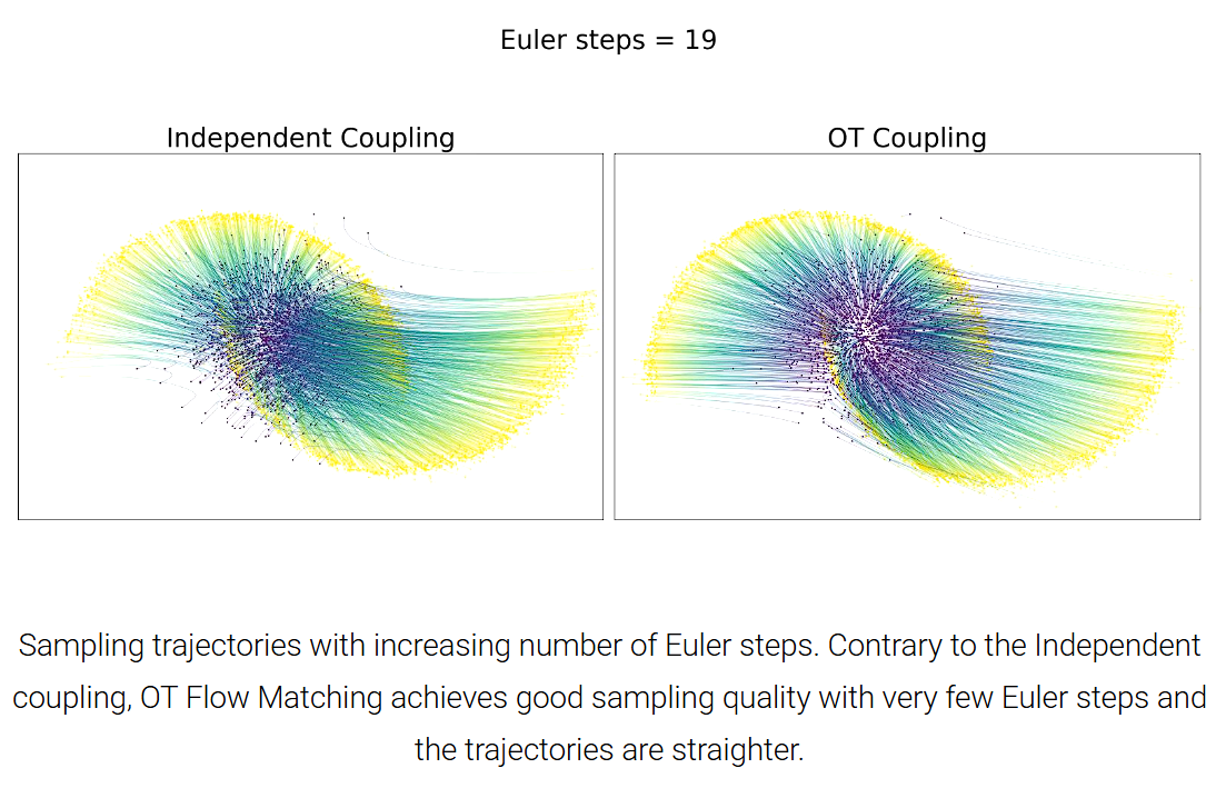
A third piece of inspiration came from recent advances in generative modeling, specifically flow matching and rectified flows. In these frameworks, Conditional Optimal Transport (CondOT) has been used to construct continuous transformations between distributions in a way that respects underlying geometry. This showed us that OT is not just a mathematical curiosity, but a practical and scalable tool for studying representation dynamics in high-dimensional spaces.
These three perspectives: the compression principle of information theory, the geometric ruler of optimal transport, and the scalable implementations from flow-based models came together to shape our approach.
Optimal Transport as a Geometric Lens on Transformer Representations
To analyze how representations evolve across layers in a neural network, we need a measure of “distance” between two sets of high-dimensional points. Traditional metrics such as Euclidean or Cosine distance can track changes at the level of individual vectors, but they fall short in capturing the collective, structural shift of the entire representation distribution. This motivates the use of Optimal Transport (OT).
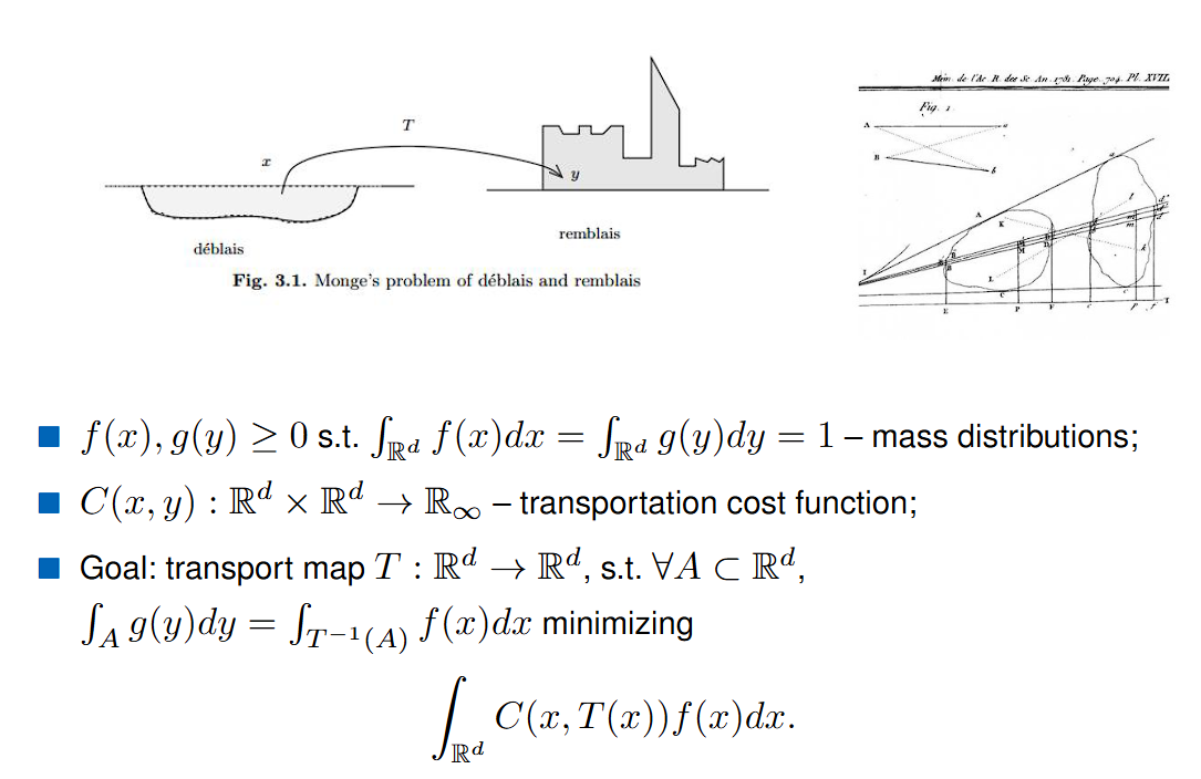
Monge’s Formulation: The Earth Mover’s Problem
The OT problem dates back to Gaspard Monge (1781), who posed it as a question of logistics: How can we move a pile of earth (distribution $P$) to fill a hole of another shape (distribution $Q$) at minimal cost?
Formally, let $P$ and $Q$ be probability distributions over a space $\mathcal{X}$. Monge’s formulation asks us to find a transport map $T:\mathcal{X}→\mathcal{X}$ such that pushing forward $P$ by $T$ gives $Q$: $T_\sharp P = Q$
and the goal is to minimize the total cost of transport:
$$ \inf_{T: T_\sharp P = Q} \int_{\mathcal{X}} c(x, T(x)) , dP(x) $$
where $c(x,y)$ is the cost of moving one unit of mass from $x$ to $y$.
While elegant, Monge’s formulation is highly restrictive: it requires a deterministic map $T$, which may not exist if mass must be split.
Kantorovich’s Relaxation: Probabilistic Transport
Leonid Kantorovich (1942) introduced a relaxation that makes OT much more flexible. Instead of searching for a transport map, he considered transport plans: joint probability distributions $\gamma(x, y)$ on $\mathcal{X} \times \mathcal{X}$ whose marginals are $P$ and $Q$. Intuitively, $\gamma(x, y)$ describes how much mass at location $x$ is assigned to location $y$.
The problem becomes: $$ \inf_{\gamma \in \Pi(P, Q)} \int_{\mathcal{X} \times \mathcal{X}} c(x, y) , d\gamma(x, y) $$
where $\Pi(P, Q)$ is the set of all valid couplings of $P$ and $Q$.
With $c(x, y) = |x-y|^2$, this gives us the 2-Wasserstein distance: $$ W_2^2(P, Q) = \inf_{\gamma \in \Pi(P, Q)} \int_{\mathcal{X} \times \mathcal{X}} |x-y|^2 , d\gamma(x, y) $$ This is a true metric on the space of probability distributions, sensitive to geometry, and often interpreted as the minimal “work” needed to transform one distribution into another.
Making OT Practical: Sinkhorn Regularization
Computing the exact Wasserstein distance is computationally expensive in high dimensions. To make it tractable, we adopt entropic regularization, which adds a penalty term based on the entropy of the transport plan: $$ OT_\varepsilon(P, Q) = \min_{\gamma \in \Pi(P, Q)} \Big( \sum_{i,j} \gamma_{ij} C_{ij} - \varepsilon H(\gamma) \Big), \quad H(\gamma) = - \sum_{i,j} \gamma_{ij} \log(\gamma_{ij}) $$
Here, $C$ is the cost matrix where $C_{jk} = | h_i^{(j)} - h_{i+1}^{(k)} |^2$, and $\varepsilon > 0$ is the regularization parameter.
This regularized version can be solved efficiently with the Sinkhorn–Knopp algorithm, yielding what is commonly called the Sinkhorn distance. In practice, this makes OT scalable to the high-dimensional distributions we encounter in neural networks. We utilize the Python Optimal Transport (POT) library for this computation. This method is not only faster but also statistically more robust for high-dimensional data, making it the ideal choice for our analysis.
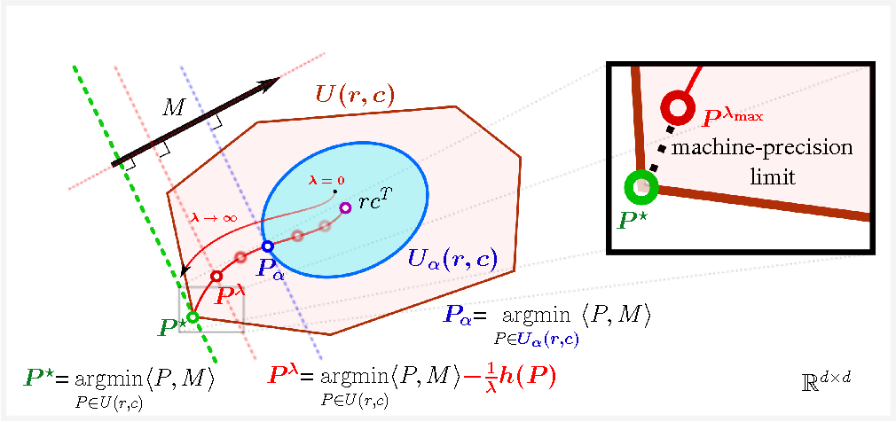
This figure illustrates how entropic regularization makes optimal transport (OT) computation fast and stable - from the paper Sinkhorn Distances: Lightspeed Computation of Optimal Transport. The classical OT solution $P^\star$ (green) lies at a sharp vertex of the transport polytope, making it expensive to compute. By adding an entropy term, Cuturi smoothed the problem, shifting the solution into the interior (red, $P^\lambda$), where it can be efficiently found using Sinkhorn iterations. As $\lambda \to 0$, the solution approaches the maximum-entropy independent coupling $rc^T$ (blue), and as $\lambda \to \infty$, it recovers the true OT solution. In practice, the Sinkhorn distance provides a controllable approximation that trades exactness for lightspeed computation.
Calculating Representation Distance with Optimal Transport
To apply optimal transport (OT) to transformer activations, we treat the problem as comparing two distributions: the representation at layer $L_i$ and the representation at the next layer $L_{i+1}$. The process unfolds in several steps:
1. Form empirical distributions: For a given batch of inputs, we collect the activation vectors at layer $L_i$, denoted ${x_1, \dots, x_n}$, and the activation vectors at layer $L_{i+1}$, denoted ${y_1, \dots, y_m}$. These two sets of vectors serve as empirical samples from distributions $P_n$ and $Q_m$.
2. Compute the cost matrix:
We construct a cost matrix $C \in \mathbb{R}^{n \times m}$, where each entry corresponds to the squared Euclidean distance between a source activation and a target activation: $C_{jk} = | x_j - y_k |^2_2$
This captures the pairwise “transport cost” between activations across adjacent layers.
3. Calculate the Sinkhorn distance:
Using the cost matrix $C$ and uniform probability weights for both empirical distributions, we compute the entropically regularized OT cost via the Sinkhorn algorithm. The resulting scalar value is what we call the OT distance between layer $L_i$ and $L_{i+1}$. Intuitively, this number reflects the geometric “work” required to reshape the distribution of activations from one layer into the next.
4. Repeat across the network:
We apply this procedure to every adjacent pair of layers in the model, yielding a full profile of OT distances across depth.
5. Compare across training:
Finally, we run the same analysis at different stages of training — both on randomly initialized (untrained) models and fully trained models. This lets us isolate the structural changes in representation flow that emerge specifically as a result of learning.
Research Findings and Analysis
The Learned Strategy of the Trained Model
When we examined the OT distances across layers in a trained model, a clear pattern emerged: the pathway of representations is not uniform but instead follows a distinct U-shaped profile. This suggests that the model organizes its internal computations into three functional phases:
1. Encoding Phase (Initial Layers):
The largest geometric transformations happen at the very beginning. The OT distance spikes between the first few layers, reflecting the effort needed to project raw embeddings into the model’s internal representational space. Soon after, this cost drops sharply, signaling that the network quickly consolidates the most important input features.
2. Refinement Phase (Middle Layers):
Once the initial heavy lifting is done, the model enters a long, stable region where OT distances remain low. Here, the network is no longer radically reshaping the geometry; instead, it is subtly refining and recombining the features it has already extracted. This stage resembles iterative reasoning, where abstract patterns are composed with relatively little geometric “work.”
3. Decoding Phase (Final Layers):
The final transition is dramatic: OT distance spikes once again at the output end of the model. This sharp increase reflects the transformation of the abstract internal state into the final task-specific output space. In other words, the last layer acts as a specialized projection head that carries the most geometrically significant burden of all.
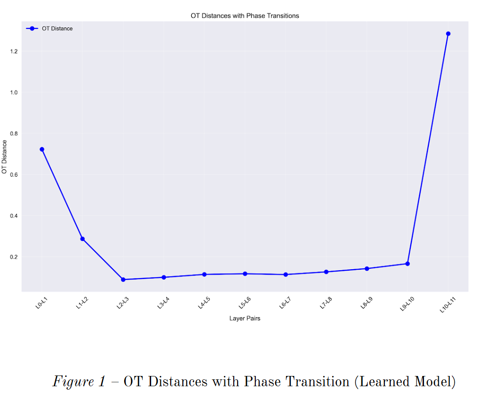
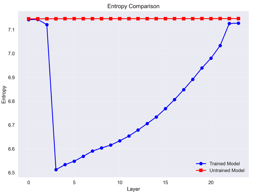
Interestingly, this three-phase pattern aligns with how the model manages representation entropy. Just as OT distances follow a U-shape, entropy plunges after the initial encoding, bottoms out in the middle layers, and rises again as the model projects into the output space. This suggests that the model has effectively learned to create an information bottleneck: compressing inputs into low-entropy, task-relevant states in the middle layers before expanding them for the final output.
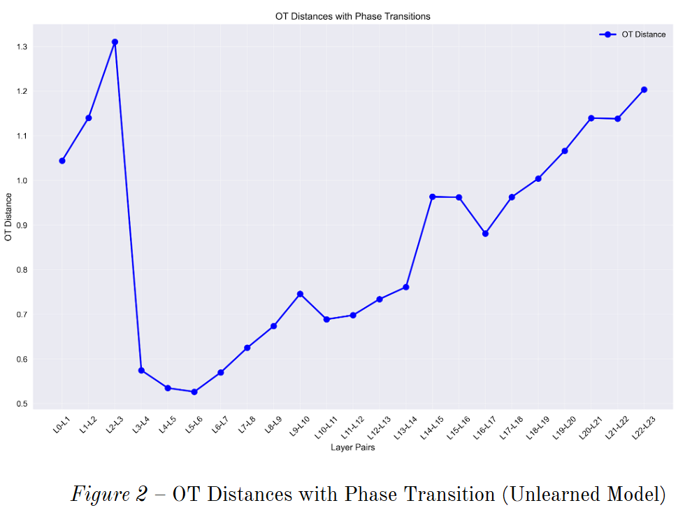
The Random Walk of the Untrained Model
The story looks very different in an untrained model. Without learning, the OT profile lacks any structured phases. Distances are uniformly high, noisy, and erratic across all layers. Every layer appears to perform a large, random transformation on its input, with no clear signs of consolidation or refinement.
Entropy dynamics tell a similar story. Instead of showing a bottleneck, entropy in the untrained model collapses abruptly at the start, then steadily increases without structure, essentially reflecting noise accumulation. This chaotic trajectory is best described as a random walk through representation space — in sharp contrast to the purposeful, three-phase strategy of the trained model.
The Emergence of the Information Bottleneck: A comparison of layer-wise representation entropy reveals that the trained model (blue) learns to compress information into a low-entropy state for refinement. In contrast, the untrained model (red) remains in a state of high disorder, demonstrating that the bottleneck is a learned, not inherent, property of the architecture.
Future Work and Experiments
- Exploring Universality and Scalability
Different Architectures: We suggest testing whether this U-shaped profile appears in other architectures. An experiment could apply this OT analysis to: Vision Transformers (ViTs), BERT-style encoder-only models, or T5-style encoder-decoder models to see if this “signature of learning” is a universal trait of transformers.
Scaling Laws: How does the geometry change with model size? One could plot the OT curves for a family of models to see if the “refinement valley” gets deeper or longer as model capability increases. This would connect the geometric view to the well-known scaling laws.
Task-Specific Dynamics: Analyze OT and entropy for models fine-tuned on different tasks (translation, summarization, reasoning) to see if the structure adapts.
- Connecting Geometry to Model Behavior
Emergent Abilities: The GSM8K dataset tests mathematical reasoning, an emergent ability. A fascinating experiment would be to track the OT profile during training. At the specific training step where the model’s accuracy on a task suddenly improves, is there a corresponding sudden change in the geometric profile, like the formation of the information bottleneck?
Fine-Tuning vs. Pre-training: Analyze and compare the OT profile of a pre-trained foundation model with its profile after being fine-tuned on a specific task. The hypothesis would be that pre-training establishes the deep U-shape, while fine-tuning primarily modifies the final “decoding” layers. This would provide geometric evidence for how transfer learning works.
Acknowledgements
I would like to thank Apart Research, PIBBSS, and Timaeus for hosting the Apart AI Safety x Physics Challenge 2025, which initiated this project. I am also grateful to Sunishka Sharma (Adobe), Janhavi Khindkar (IIIT Hyderabad), and Vishnu Vardhan Lanka (Independent Researcher), who were members of my team.
Apart Labs provided funding and support for this research, without which this work would not have been possible. I would also like to thank Jesse Hoogland, Ari Brill, and Esben Kran for providing insightful feedback on our initial draft.