Go With The Flow

Flow-based generative models are starting to turn heads as a cool alternative to traditional diffusion methods for things like image and audio generation. What makes them stand out is how they learn smooth, efficient paths to transform one distribution into another—basically a neat and mathematically solid way to generate data. They’ve been getting a lot more buzz lately, especially after Black Forest Labs dropped their FLUX models and SD3.5 model by Stability AI. That success has brought fresh attention to the earlier ideas behind Rectified Flows, which first popped up at ICLR 2023.

This wave of renewed interest is pushing researchers to rethink how we model generative processes—not just as noisy reversals but as guided, purposeful flows through data space. Unlike diffusion models that slowly denoise data step by step, flow-based models aim to learn the exact path from noise to structure in one go, which can make generation faster and more controllable. Plus, with growing support from recent papers and open-source projects, it’s becoming easier for developers and researchers to experiment with these models and push them into new creative and scientific applications.

So What’s a Flow?

Imagine you’re watching a river flow downstream. At every point, the water has a direction and speed—it’s not just sitting still. Now picture a tiny leaf floating on that river. As time passes, the river carries the leaf smoothly along a path. That motion—the direction the leaf moves at each point in time—is what we’d call a flow.

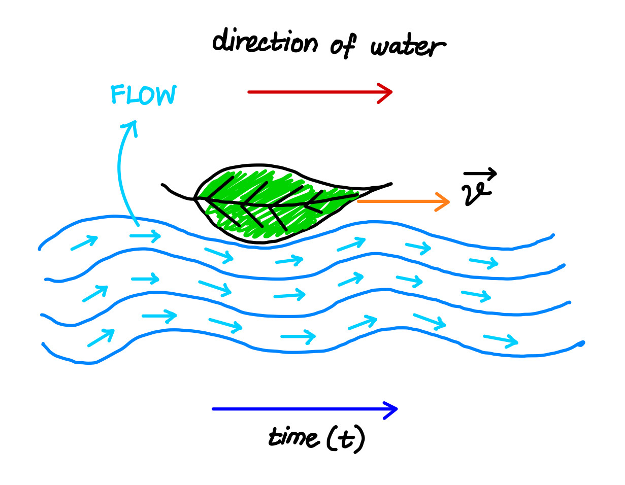
In the world of generative AI, we can think of data points like that little leaf, and the flow is a kind of invisible force field that guides how we transform one kind of data (say, pure noise) into another (like a realistic image). Instead of just jumping from noise to image, the model learns how to gradually reshape the randomness into structure, just like the river reshapes the leaf’s position as it moves.

So, just like in a river or a gust of wind, every point in space has a little arrow—a velocity vector—that tells tiny particles where to move. And just like how water currents or wind patterns can change over time and space, our model’s “flow field” can also depend on both position and time.

Flow matching taps into this idea by trying to learn those natural movement patterns. It’s like asking at every moment, “If this data point were a leaf on a river, which direction should it drift right now?” The model doesn’t just guess the final destination—it learns the smooth path each point should follow through the data space.

A Quick Linear Algebra Refresher

Before we dive deeper into the mathematical intuition behind flows and how flow-based models actually work, let’s hit pause and take a quick detour to understand what is a Jacobian and the Change of Variables theorem.

Given a function of mapping a $n$-dimensional input vector $\mathbf{x}$ to a $m$-dimensional output vector, $f : \mathbb{R}^n \mapsto \mathbb{R}^m$, the matrix of all first-order partial derivatives of this function is called the Jacobian matrix, $\mathbf{J}$, where one entry on the $i$-th row and $j$-th column is
$$ \mathbf{J}_{ij} = \frac{\partial f_i}{\partial x_j} $$ The Jacobian matrix looks like: $$ J = \begin{bmatrix} \displaystyle \frac{\partial f_1}{\partial x_1} & \cdots & \displaystyle \frac{\partial f_1}{\partial x_n} \ \vdots & \ddots & \vdots \ \displaystyle \frac{\partial f_m}{\partial x_1} & \cdots & \displaystyle \frac{\partial f_m}{\partial x_n} \end{bmatrix} $$

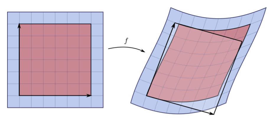
The Jacobian tells us how a function transforms space locally—it shows how small changes in input affect each output. It acts like a map of sensitivities and stretching, and its determinant measures how much the function expands or contracts space at a point.

The determinant is a single number that summarizes certain properties of a square matrix. You can only compute it for square matrices—that is, matrices with the same number of rows and columns.

At a high level, the determinant tells us how much a matrix stretches or squashes space.
You can think of it as measuring the “volume change” caused by the matrix when it transforms data. For an $n \times n$ matrix $M$, the determinant is calculated as:

$$ \det M = \begin{vmatrix} a_{11} & a_{12} & \cdots & a_{1n} \ a_{21} & a_{22} & \cdots & a_{2n} \ \vdots & \vdots & \ddots & \vdots \ a_{n1} & a_{n2} & \cdots & a_{nn} \end{vmatrix} = \sum_{j_1 j_2 \cdots j_n} (-1)^{\tau(j_1 j_2 \cdots j_n)} a_{1j_1} a_{2j_2} \cdots a_{nj_n} $$

This sum runs over all possible permutations of column indices $j_1, j_2, \dots, j_n$.
The function $\tau(\cdot)$ gives the sign of each permutation (+1 or -1), depending on how “twisted” it is.

Why is the determinant useful?

• If $\det(M) = 0$, the matrix flattens space in some direction—it’s not reversible. This means the matrix is not invertible (it’s singular).
• If $\det(M) \ne 0$, then the matrix preserves some volume, and is invertible.

A neat property of determinants:
If you multiply two square matrices, their determinants also multiply:

$$ \det(AB) = \det(A) \cdot \det(B) $$

Change of Variables Theorem (for Density Estimation)

At it’s core Change of Variable theorem tells us how a probability density changes when you transform the variable it’s defined on.

Let’s go over the change of variable theorem in the context of probability density estimation, starting with the simple case of a single variable.

One-Dimensional Case

Suppose we have a random variable $z$ with known density $\pi(z)$, and we define a new variable $x = f(z)$ using a 1-to-1 invertible function $f$. This means $z = f^{-1}(x)$.
Now we want to find the unknown density of $x$, denoted $p(x)$.

Using the fact that probabilities must sum to 1:

$$ \int p(x) \ dx = \int \pi(z) \ dz = 1 $$

To convert densities between variables, we apply the change of variables formula:

$$ p(x) = \pi(z) \left| \frac{dz}{dx} \right| = \pi(f^{-1}(x)) \left| \frac{d f^{-1}}{dx} \right| = \pi(f^{-1}(x)) \left| (f^{-1})’(x) \right| $$

Here, $\left| \frac{df^{-1}}{dx} \right|$ captures how the space is stretched or squashed during transformation.

Think of the integral $\int \pi(z) , dz$ as adding up many thin rectangles. Each rectangle has Width $\Delta z$ and Height $\pi(z)$. When we substitute $z = f^{-1}(x)$, we’re essentially changing the coordinates. The width becomes:$$ \Delta z = \left( f^{-1}(x) \right)’ \Delta x $$So, the scaling factor $\left| (f^{-1}(x))’ \right|$ tells us how the density stretches when changing variables.

Multivariable Case

For higher dimensions, the concept extends using the Jacobian determinant.

Let: $$ z \sim \pi(z), \quad x = f(z), \quad z = f^{-1}(x) $$

Then the density transforms as:

$$ p(x) = \pi(z) \left| \det \frac{dz}{dx} \right| = \pi(f^{-1}(x)) \left| \det \frac{d f^{-1}}{dx} \right| $$

Here, $\det \frac{\partial f}{\partial x}$ is the Jacobian determinant of the function $f$.

Normalizing Flows

Normalizing Flows is a method for turning a simple probability distribution (like a Gaussian) into a complex one by applying a sequence of invertible and differentiable transformations.

Normalizing Flows learn an invertible mapping $f: \mathcal{X} \rightarrow \mathcal{Z}$ ; where $\mathcal{X}$ is the data distribution and $\mathcal{Z}$ is a chosen latent distribution.

Let:

$$ x = f_\theta(z) = f_k \circ \cdots \circ f_2 \circ f_1(z) $$

where each $f_i$ is invertible (bijective).

We define:

$$ f: \mathcal{Z} \rightarrow \mathcal{X}, \quad \text{where } f \text{ is invertible} $$

Let $p_\theta(x)$ be the probability density over $x$, with $z \in \mathcal{Z}$.

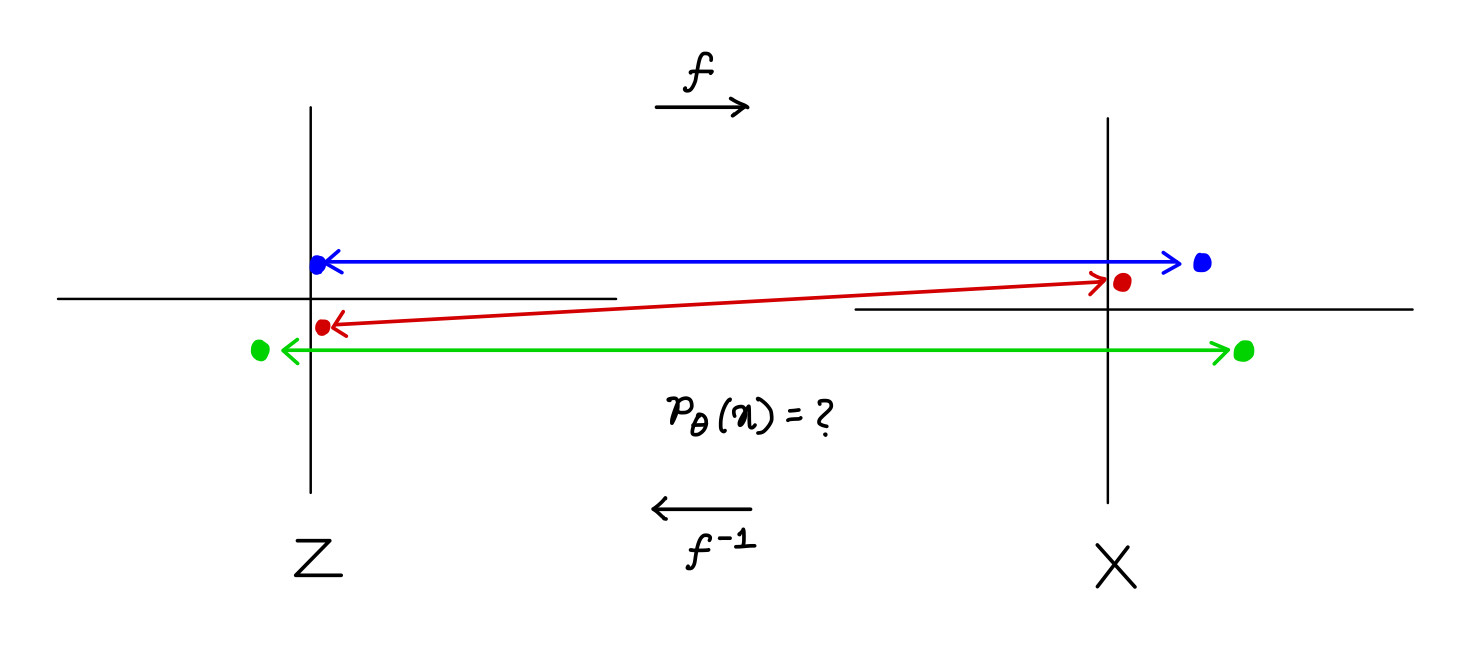
Change of Variable Formula:

$$ p_\theta(x) = p_\theta(f^{-1}(x)) \left| \det \left( \frac{\partial f^{-1}(x)}{\partial x} \right) \right| $$

If we replace $f^{-1}(x)$ with $z$, the formula becomes:

$$ p_\theta(x) = p_\theta(z) \left| \det \left( \frac{\partial z}{\partial x} \right) \right| $$ Finally:

$$ p_\theta(x) = p_\theta(z) \prod_{i=1}^{k} \left| \det \left( \frac{\partial f_i^{-1}}{\partial z_i} \right) \right| = p_\theta(z) \left| \det \left( \frac{\partial f^{-1}}{\partial x} \right) \right| $$

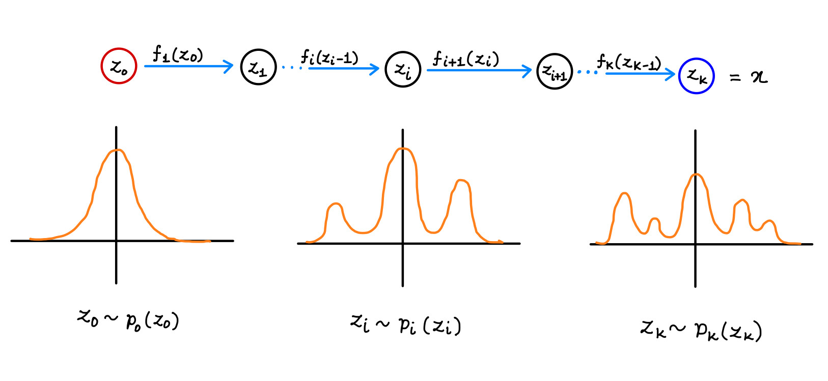
The sequence of transformations applied to random variables, expressed as:

$$ z_i = f_i(z_{i-1}) $$

is called the flow. When this sequence forms a chain of distributions $\pi_i$, the entire process is referred to as a normalizing flow. For each transformation function $f_i$ in the flow to be usable in practice, it must meet two key criteria:

1. It must be easily invertible.
2. Its Jacobian determinant must be efficient to compute.

Why Are Normalizing Flows Called “Normalizing” Flows?

Normalizing Flows refer to the process of transforming probability distributions while preserving normalization—i.e., ensuring they remain valid probability distributions. The change of variables formula ensures that the probability density is adjusted (or “normalized”) correctly during this transformation. This adjustment is what allows the transformed distribution to stay normalized—hence the name “Normalizing Flows”.

Exact Log-Likelihoods with Normalizing Flows

One of the key advantages of Normalizing Flows is that they allow us to compute exact log-likelihoods, which is rare for most generative models.

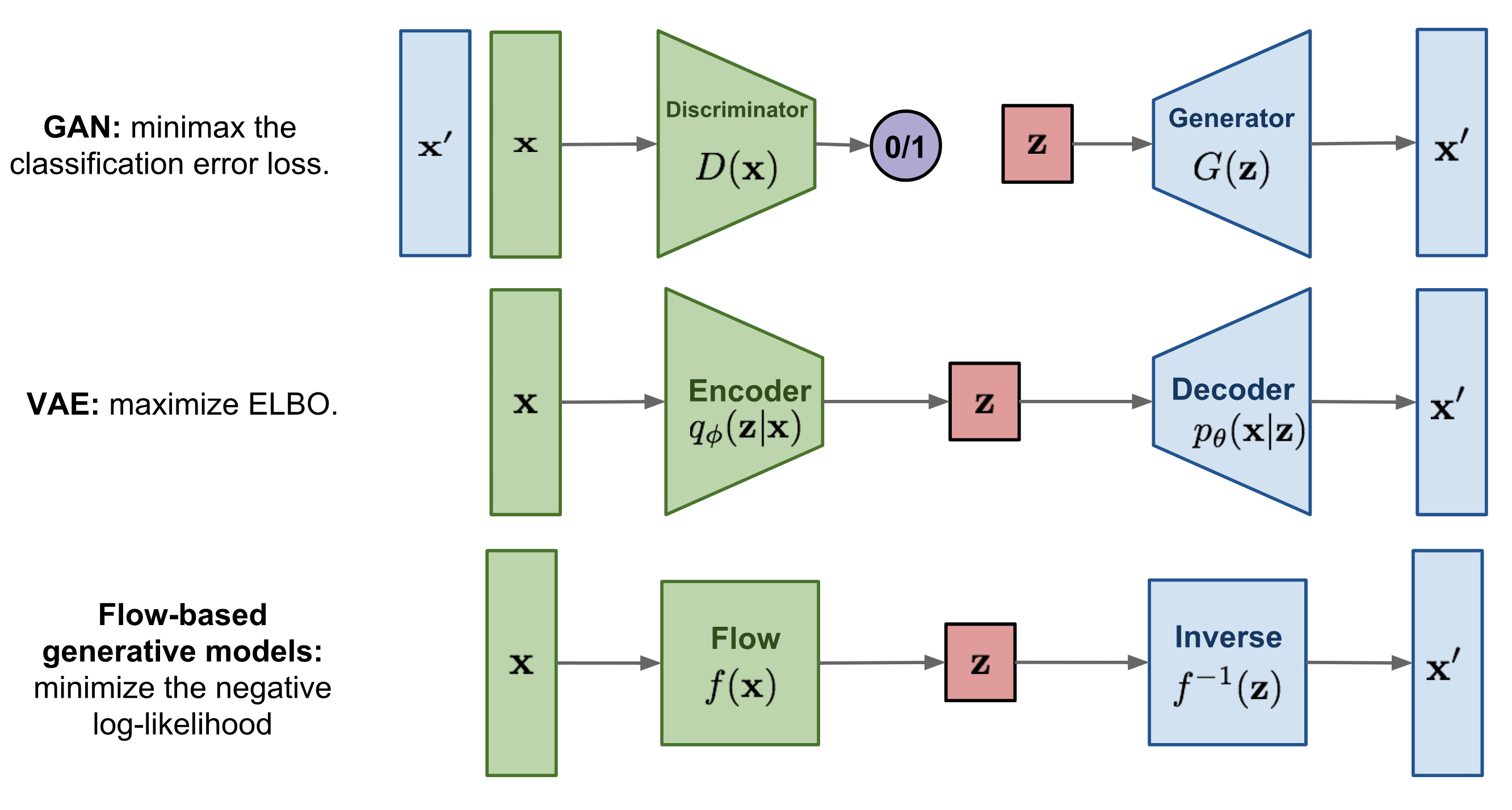
Variational Autoencoders (VAEs)

• Provide only a lower bound on the log-likelihood (ELBO).
• Use an approximate posterior $q_\phi(z \mid x)$

Generative Adversarial Networks (GANs)

• Do not support log-likelihood evaluation.
• Do not provide latent variable inference.

Normalizing Flows

With normalizing flows, we can compute:

$$ \log p_\theta(x) = \log p_\theta(z) + \sum_{i=1}^K \log \left| \det \left( \frac{\partial f_i^{-1}}{\partial z_i} \right) \right| $$

• Allows for exact log-likelihood evaluation.
• Also enables exact posterior inference via the invertible transformation $z = f^{-1}(x)$

Flow Matching - A Deep Dive

Given a training dataset sampled from a target distribution $q$ over $\mathbb{R}^d$, the goal is to learn a generative model that can produce new samples from $q$. To achieve this, Flow Matching (FM) constructs a probability path $(p_t)_{0 < t < 1}$ that transitions from a known source distribution $p_0 = p$ to the target distribution $p_1 = q$, where each $p_t$ is a distribution over $\mathbb{R}^d$.

Flow Matching works by training a velocity field—a neural network that estimates the instantaneous velocity of samples along this path. This field is later used to transport samples from the source $p_0$ to the target $p_1$ by solving a differential equation.

After training, generating a new sample from the target distribution $X_1 \sim q$ involves:

1. Sampling an initial point $X_0 \sim p$, and
2. Solving the Ordinary Differential Equation (ODE) guided by the learned velocity field.

Why to solve the ODE? Given a starting point $X_0$ ODE tells you how to move it to $X_1$.

A flow $\psi_t : \mathbb{R}^d \rightarrow \mathbb{R}^d$ (represented by the square grid) is defined through a velocity field $u_t : \mathbb{R}^d \rightarrow \mathbb{R}^d$, visualized here using blue arrows. This velocity field dictates how every point moves instantaneously across space. The three images illustrate how the grid is progressively deformed at different time steps $t$.

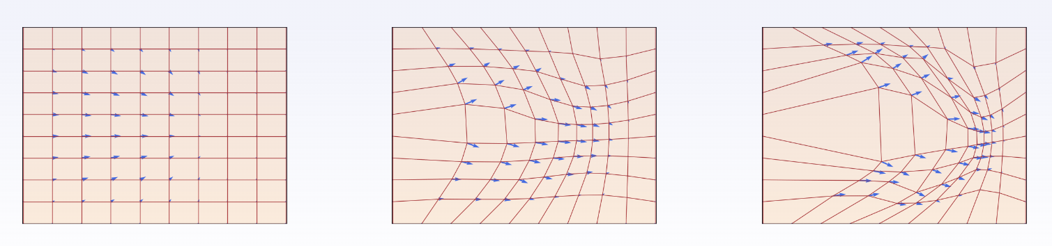
The objective of generative flow modeling is to learn a flow $\psi_t$ such that:

$$ X_1 = \psi_1(X_0) \sim q, $$

where $X_0$ is sampled from a simple source distribution (e.g., Gaussian), and $q$ is the target data distribution.

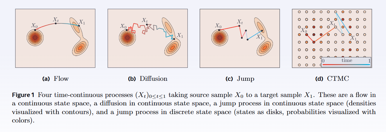
Note: Flow and Diffusion Models

Both Flow Models and Diffusion Models generate samples by evolving a random variable over time, starting from a simple initial distribution.

Flow Model

Initialize:
$$ X_0 \sim p_{\text{init}} \quad \text{(e.g., Gaussian)} $$ Evolve using an ODE:
$$ dX_t = u_t^\theta(X_t)\ dt $$

• $u_t^\theta$ is a neural network that defines a time-dependent vector field.
• The evolution is deterministic (no randomness).

Diffusion Model

Initialize:
$$ X_0 \sim p_{\text{init}} $$ Evolve using an SDE: $$ dX_t = u_t^\theta(X_t)\ dt + \sigma_t\ dW_t $$

• $u_t^\theta$ is again a neural network vector field.
• $\sigma_t$ is the diffusion coefficient.
• $dW_t$ is a Wiener process (i.e., standard Brownian motion).
• The evolution is stochastic, involving both learned dynamics and noise.

Constructing the Training Target for Flow Models

Typically, we train the model by minimizing a mean squared error:

$$ L(\theta) = \left| u_t^\theta(x) - u_t^{\text{target}}(x) \right|^2 $$

Here, $u_t^{\text{target}}(x)$ is the training target we want the model’s prediction $u_t^\theta(x)$ to match.

In standard regression or classification, the training target is usually a label. But in this case, we don’t have labels. So instead, we need to derive the training target ourselves.

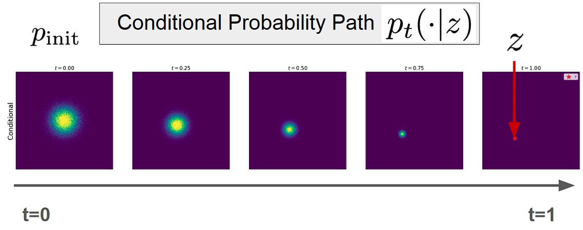
Conditional Probability Path

Dirac Distribution:

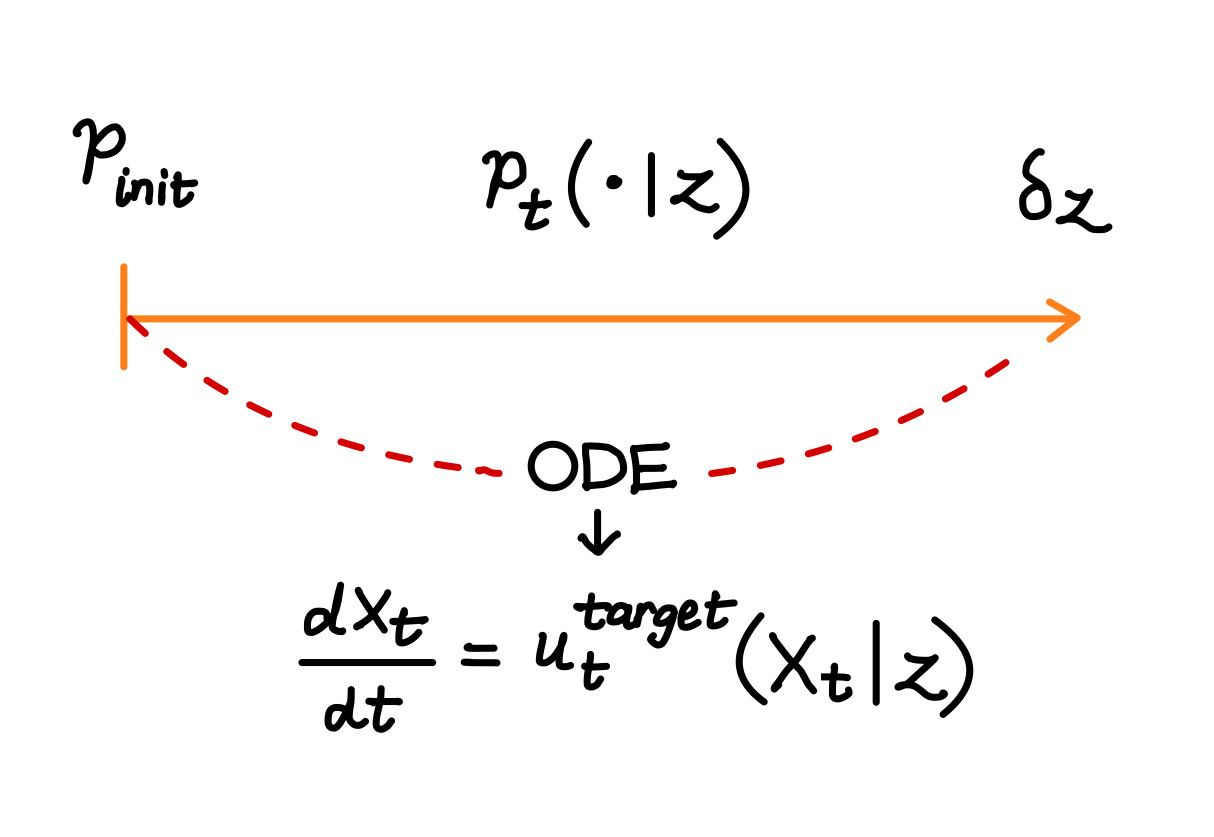
Let: $z \in \mathbb{R}^d, \quad \delta_z \Rightarrow X = z$ Here, $\delta_z$ is the Dirac distribution, which assigns all probability mass to the single point $z$. This implies $X$ takes the exact value $z$.

We define a conditional probability path $p_t(\cdot \mid z)$ such that $p_t(\cdot \mid z)$ is a distribution over $\mathbb{R}^d$ The path starts at: $p_0(\cdot \mid z) = p_{\text{init}}$ and ends at $p_1(\cdot \mid z) = \delta_z$ This means we begin from an initial distribution and evolve it into a Dirac delta centered at $z$.

Example : Gaussian Probability Path - An example of such a conditional path is a Gaussian with time-varying mean and variance: $\mathcal{N}(\alpha_t z,\ \beta_t^2 I_d)$. This describes a path where samples are centered around $\alpha_t z$ and the uncertainty (spread) is controlled by $\beta_t^2$.

Note : Conditional means per single data point and marginal means across distribution of data points

Conditional Vector Field

We define a target conditional vector field:

$$ u_t^{\text{target}}(x \mid z), \quad \text{for } 0 \leq t \leq 1,\ x, z \in \mathbb{R}^d $$

such that: $$ X_0 \sim p_{\text{init}}, \quad \frac{d}{dt}X_t = u_t^{\text{target}}(X_t \mid z) \quad \Rightarrow \quad X_t \sim p_t(\cdot \mid z) ;\quad 0 \leq t \leq 1 $$

• $X$ is the variable of interest (what we want to evolve or sample).
• $z$ is the conditioning variable.
• The vector field $u_t^{\text{target}}(x \mid z)$ is time-dependent (indexed by $t$), and it guides the evolution of $X$ conditioned on $z$.

If we start with samples from a known distribution and move them using this conditional vector field, then the distribution of the evolved particles at time $t$ will follow the conditional target distribution $X_t \sim p_t(x \mid z)$.

Start by sampling $X_0$ from an initial distribution $p_{\text{init}}$. Then, evolve the samples over time using the conditional vector field $u_t^{\text{target}}(x \mid z)$ by solving the following ODE:

$$ \frac{dX_t}{dt} = u_t^{\text{target}}(X_t \mid z) $$

As the system evolves, at any time $t$, the samples $X_t$ should follow the desired conditional probability distribution: $$ X_t \sim p_t(x \mid z) $$

Marginal Probability Path

We define the marginal path $p_t$ as the marginalization over conditional distributions.

Given:

• $z \sim p_{\text{data}}$ and $X \sim p_t(\cdot \mid z)$ -> then $X \sim p_t$

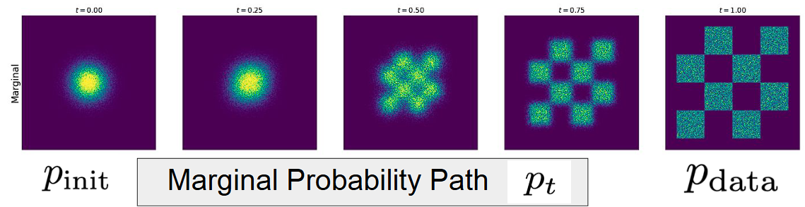
To obtain the marginal distribution $p_t(X)$, we integrate over $z$:

$$ p_t(X) = \int p_t(X \mid z) \ p_{\text{data}}(z) \ dz $$

We define the probability path with:

• $p_0 = p_{\text{init}}$ (start from noise)
• $p_1 = p_{\text{data}}$ (end at real data)

This defines a smooth transformation from noise → data over time, as illustrated in the figure with intermediate distributions $p_t$ between $t = 0$ and $t = 1$

Marginal Vector Field

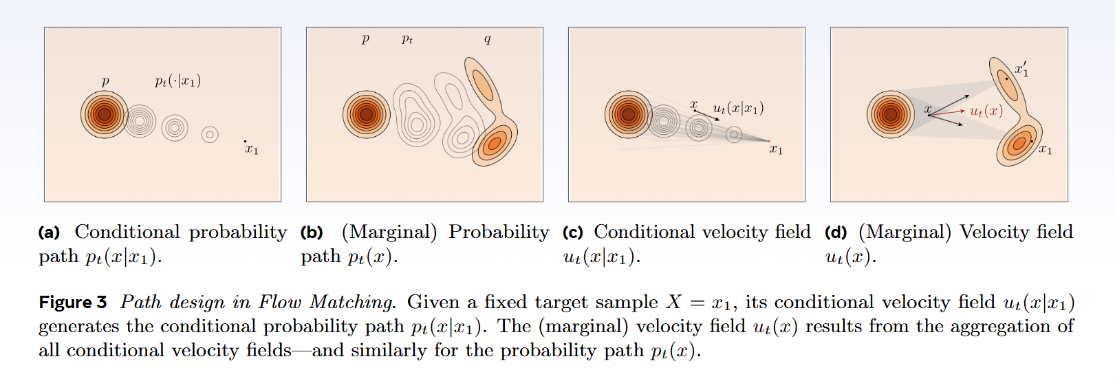
We can define the marginal target vector field $u_t^{\text{target}}(x)$ by averaging the conditional vector field $u_t^{\text{target}}(x \mid z)$ weighted by the joint distribution:

$$ u_t^{\text{target}}(x) = \int u_t^{\text{target}}(x \mid z) \cdot \frac{p_t(x \mid z) \cdot p_{\text{data}}(z)}{p_t(x)} \ dz $$

This equation uses the conditional vector field and transforms it into a marginal one over x. This satisfies: If we sample from the initial distribution and evolve using this marginal vector field:

$$ X_0 \sim p_{\text{init}}, \quad \frac{d}{dt} X_t = u_t^{\text{target}}(X_t) $$

Then the samples $X_t$ follow the marginal distribution:

$$ X_t \sim p_t \quad \text{for } t \in [0, 1] $$

At $t = 1$, we reach the target:

$$ X_1 \sim p_{\text{data}} $$

This method is often referred to as the “Marginalization Trick”, where we compute a marginal vector field $u_t^{\text{target}}(x)$ given the conditional one $u_t^{\text{target}}(x \mid z)$.

Conditional & Marginal Score Function

In generative modeling, a score function refers to the gradient of the log-probability with respect to the input. It points in the direction where the data density increases—useful for guiding the sampling process.

1. Conditional Score

$$ \nabla_x \log p_t(x \mid z) $$ Represents the gradient of the log-density of $x$ given a conditioning variable $z$. It tells us how likely $x$ is, assuming we already know $z$.

2. Marginal Score

$$ \nabla_x \log p_t(x) $$ Represents the gradient of the marginal log-density of $x$, where $z$ is integrated out. It is used in unconditional models that learn the overall data distribution without conditioning. Central to score-based diffusion models and other likelihood-free approaches.

Flow Matching

Now that we’ve covered the core ideas behind flow models—like what a flow is, how normalizing flows work, and the roles of conditional and marginal probability paths and vector fields—let’s dive into what Flow Matching actually is.

The goal of Flow Matching is to learn a neural vector field $u_t^\theta$ that closely matches the target vector field $u_t^{\text{target}}$:

$$ u_t^\theta \approx u_t^{\text{target}} $$

Flow Matching Loss

The objective in flow matching is to minimize the difference between the learned vector field $u_t^\theta(x)$ and the target vector field $u_t^{\text{target}}(x)$. The ideal loss function is:

$$ \mathcal{L}_{\text{fm}}(\theta) = \mathbb{E} \left[ \left| u_t^\theta(x) - u_t^{\text{target}}(x) \right|^2 \right] $$

To evaluate this loss (in theory), we would:

• Sample $t \sim \text{Uniform}[0, 1]$
• Sample $z \sim p_{\text{data}}$ (a real data point)
• Sample $x \sim p_t(\cdot \mid z)$ from the conditional path

The challenge is that we cannot directly compute this loss, because the true target vector field $u_t^{\text{target}}(x)$ is unknown or intractable. So what’s the solution? Conditional Flow Matching Loss!

Conditional Flow Matching Loss

We define the Conditional Flow Matching (CFM) loss as:

$$ \mathcal{L}_{\text{cfm}}(\theta) = \mathbb{E} \left[ \left| u_t^\theta(x) - u_t^{\text{target}}(x \mid z) \right|^2 \right] $$

Where:

• $t \sim \text{Uniform}[0, 1]$
• $z \sim p_{\text{data}}$ (draw a data sample)
• $x \sim p_t(\cdot \mid z)$ (draw from conditional probability path)

Theorem:

There exists a constant $c > 0$ (independent of $\theta$) such that:

$$ L_{\text{fm}}(\theta) = L_{\text{cfm}}(\theta) + c $$

This means minimizing the conditional loss is equivalent (up to a constant) to minimizing the original flow matching loss.

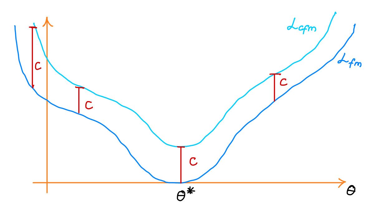
Key Consequences

1. The minimizer $\theta^*$ of $\mathcal{L}_{\text{cfm}}$ satisfies:

$$ u_t^{\theta^*} = u_t^{\text{target}} $$

2. The gradients are the same:

$$ \nabla_\theta L_{\text{cfm}}(\theta) = \nabla_\theta L_{\text{fm}}(\theta) $$

So **Stochastic Gradient Descent (SGD)** behaves the same for both losses and the training trajectories will not differ. All we need to do is minimize a simple mean squared error loss, which is much easier to optimize than adversarial objectives like those in GANs (which require min-max optimization).

Flow Matching Training Procedure (General)

Given:

• A dataset of samples $z \sim p_{\text{data}}$
• A neural network $u_t^\theta$ (the learnable vector field)

Training Loop

For each mini-batch of data:

1. Sample a data example $z$ from the dataset.
2. Sample a random time $t \sim \text{Uniform}[0, 1]$.
3. Sample $x \sim p_t(\cdot \mid z)$ — from the conditional path at time $t$.
4. Compute the flow matching loss: $$ \mathcal{L}(\theta) = \left| u_t^\theta(x) - u_t^{\text{target}}(x \mid z) \right|^2 $$
5. Update model parameters $\theta$ using gradient descent on $\mathcal{L}(\theta)$.

Flow Matching Training for CondOT (Optimal Transport) Path

Given:

• A dataset of samples $z \sim p_{\text{data}}$
• A neural network vector field $u_t^\theta$

Training Procedure

For each mini-batch:

1. Sample a data example $z$ from the dataset.
2. Sample a random time $t \sim \text{Uniform}[0, 1]$.
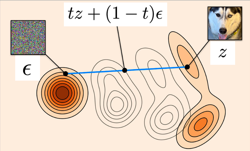
3. Sample noise $\epsilon \sim \mathcal{N}(0, I_d)$.
4. Compute: $$ x = t z + (1 - t) \epsilon $$
5. Compute the loss: $$ \mathcal{L}(\theta) = \left| u_t^\theta(x) - (z - \epsilon) \right|^2 $$
6. Update model parameters $\theta$ via gradient descent on $\mathcal{L}(\theta)$.

Rectified Flows

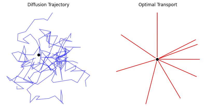
Since distributions are at the heart of statistics and machine learning, many core problems—like generative modeling and domain transfer—can be understood through the lens of finding a transport map that moves one distribution to another. Rectified Flow offers a simple way to do this by learning an ordinary differential equation (ODE), also known as a flow model, with the central idea of encouraging movement along straight paths as much as possible. This approach is closely connected to neural ODEs and stochastic differential equation (SDE) models, particularly the widely used diffusion generative models and their ODE variants.

Traditionally, there are infinitely many ODEs or SDEs that could map between two distributions, and most methods implicitly choose a trajectory without a clear principle. In contrast, rectified flow explicitly prefers ODEs whose solution paths are straight lines—what they call straight flows. This leads to a simple, principled framework that ties naturally to optimal transport theory. A major advantage is that straight flows eliminate discretization error when solving ODEs numerically, meaning rectified flows allow very fast inference—sometimes achievable in just a single Euler step. As a result, they combine the speed of one-step generative models like GANs and VAEs with the robustness and training stability of multi-step ODE/SDE-based models.

Learning Transport Maps

The Transport Mapping Problem:

Given empirical observations of two distributions $\pi_0, \pi_1$ on $\mathbb{R}^d$,
the goal is to find a transport map:

$$ T: \mathbb{R}^d \to \mathbb{R}^d $$

such that, in the infinite data limit, $Z_1 := T(Z_0) \sim \pi_1$ when $Z_0 \sim \pi_0$.
In other words, $(Z_0, Z_1)$ forms a coupling (also called a transport plan) between $\pi_0$ and $\pi_1$.

• Generative Modeling:

  • $\pi_1$ is an unknown data distribution (e.g., images),
  • $\pi_0$ is a simple known distribution (e.g., standard Gaussian).
  • The goal is to learn a nonlinear transform that maps samples from $\pi_0$ to samples from $\pi_1$.

• Transfer Modeling:

  • Both $\pi_0$ and $\pi_1$ are unknown empirical distributions.
  • The goal is to transfer data points from $\pi_0$ to $\pi_1$, or vice versa.
  • Applications include domain adaptation, transfer learning, image editing, and sim2real in robotics.

Why is Finding a Transport Map Challenging?

Given two distributions, there are infinitely many possible transport maps $T$.
The goal is to find one that transfers $\pi_0$ to $\pi_1$ and has desirable properties, such as high computational efficiency and practical simplicity

To achieve this, we often formulate the problem mathematically to impose additional desirable properties.

Optimal Transport (OT)

One canonical formulation is Optimal Transport (OT), where we seek a transport plan that minimizes a cost.

Specifically, Monge’s Optimal Transport problem is:

$$ \min_T \mathbb{E} \left[ c(T(Z_0) - Z_0) \right] \quad \text{subject to} \quad \text{Law}(Z_0) = \pi_0, \quad \text{Law}(T(Z_0)) = \pi_1 $$ where:

• $c: \mathbb{R}^d \to \mathbb{R}$ is a cost function (e.g., $c(x) = \frac{1}{2} |x|^2$),
• $\mathbb{E}\left[ c(T(Z_0) - Z_0) \right]$ measures the expected transport cost.

Think of $Z_0$ and $Z_1$ as two piles of sand, and $c(Z_1 - Z_0)$ as the cost of moving sand from $Z_0$ to $Z_1$.

However, solving the optimal transport (OT) problem remains highly challenging, especially when dealing with high-dimensional data and large-scale datasets. Developing efficient algorithms for these settings is still an open problem.

Moreover, in generative and transfer modeling, the transport cost itself is often not the primary focus — the learning performance is not directly tied to the magnitude of $Z_1 - Z_0$. While optimal transport maps do induce smoothness properties that are beneficial for learning, minimizing transport cost isn’t the ultimate goal.

Method: Rectified Flow

Rectified flow learns the transport map $T$ implicitly by constructing an
ordinary differential equation (ODE) driven by a drift force:

$$ dZ_t = v(Z_t, t) dt, \quad t \in [0, 1], \quad \text{starting from} \quad Z_0 \sim \pi_0 $$

The goal is to ensure that when we follow the ODE starting from $Z_0 \sim \pi_0$,
we end up with $Z_1 \sim \pi_1$.

The main challenge is how to construct the drift field $v$ based only on observations from $\pi_0$and $\pi_1$, typically using deep neural networks or other nonlinear approximators.

At first glance, this looks hard. One natural idea is to find $v$ by minimizing a discrepancy measure $D(\rho_1^v, \pi_1)$, where $\rho_1^v$ is the distribution of $Z_1$ after following the ODE driven by $v$ and $D(\cdot, \cdot)$ is some divergence, like KL divergence.

However, this requires:

• Repeated simulation of the ODE,
• Inferring intermediate states, which is computationally expensive,
• And the big problem: we don’t know what intermediate trajectories the ODE should travel through!

We can avoid these difficulties by exploiting the over-parameterized nature of the problem. Since we only care about matching the start ($\pi_0$) and end ($\pi_1$) distributions,
the intermediate states $\pi_t$ of $Z_t$ can be any smooth interpolation between $\pi_0$ and $\pi_1$. Thus, we can (and should) inject strong assumptions about the intermediate paths.
The simplest and most effective assumption? Straight trajectories.

Why Straight Paths?

• Theoretically: They align well with ideas from optimal transport.
• Computationally: ODEs following straight paths have zero discretization error,
  meaning they can be solved exactly or with very few numerical steps.

How Rectified Flow Works

Specifically, rectified flow works by finding an ODE to match the marginal distributions of the linear interpolation of points between $\pi_0$ and $\pi_1$.

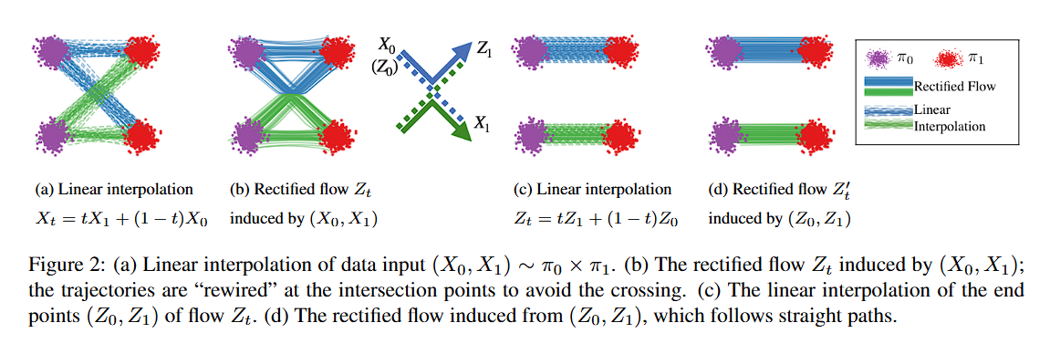
Assume we observe $X_0 \sim \pi_0$ and $X_1 \sim \pi_1$. Let $X_t$ for all $t \in [0,1]$ be the linear (geodesic) interpolation between $X_0$ and $X_1$:

$$ X_t = t X_1 + (1 - t) X_0 $$

Observe that $X_t$ follows a simple ODE that already transfers $\pi_0$ to $\pi_1$:

$$ dX_t = (X_1 - X_0)dt $$

This means that $X_t$ moves along the line direction $(X_1 - X_0)$ at a constant speed. However, this ODE is non-causal:

• The update $X_t$ depends on the final state $X_1$, which is unknown at time $t < 1$.
• When multiple trajectories cross at a point $X_t$, the direction of motion becomes ambiguous and non-unique.
• Thus, the “causal ODE” needed for simulation cannot just be the naive ODE in the equation above.

Solution: Causalizing the Interpolation

We want to “causalize” the interpolation process $X_t$ by projecting it into the space of causally simulatable ODEs:

$$ dZ_t = v(Z_t, t) dt $$

A natural way to do this is to project the velocity field onto a causal one by minimizing an L2 loss:

$$ \min_v \int_0^1 \mathbb{E} \left[ | (X_1 - X_0) - v(X_t, t) |^2 \right] dt $$

This finds a drift $v$ that approximates the ideal direction $(X_1 - X_0)$ as closely as possible at each point $(X_t, t)$.

Theoretical Solution: Conditional Expectation

The optimal drift $v(z,t)$ can be written as:

$$ v(z, t) = \mathbb{E}[X_1 - X_0 \mid X_t = z] $$

This means $v(z,t)$ is the expected direction of the lines passing through the point $z$ at time $t$. We call the ODE with this $v(z,t)$ the rectified flow induced from $(X_0, X_1)$.

In practice:

• We solve the minimization using standard optimizers like SGD.
• We parameterize $v$ with a neural network or other function approximator.
• The conditional expectation $\mathbb{E}[\cdot]$ is estimated empirically from samples $(X_0, X_1)$.

The trajectories $Z_t$ traced by rectified flow follow the same density path as the original interpolation $X_t$,
but they rewire themselves at intersections to maintain causality and avoid non-uniqueness.

Key Properties of Rectified Flow

1. The ODE trajectories $Z_t$ and the interpolation $X_t$ have the same marginal distributions for all $t \in [0, 1]$:

$$ \text{Law}(Z_t) = \text{Law}(X_t), \quad \forall t \in [0, 1]. $$

Thus, $(Z_0, Z_1)$ forms a valid coupling of the distributions $\pi_0$ and $\pi_1$.

2. The coupling $(Z_0, Z_1)$ also guarantees no larger transport cost compared to $(X_0, X_1)$ for any convex cost function $c : \mathbb{R}^d \to \mathbb{R}$:

$$ \mathbb{E} \left[ c(Z_1 - Z_0) \right] \leq \mathbb{E} \left[ c(X_1 - X_0) \right], \quad \forall \text{ convex } c. $$

• The data pair $(X_0, X_1)$ can be an arbitrary (possibly independent) coupling of $\pi_0$ and $\pi_1$
• Typically, $(X_0, X_1) \sim \pi_0 \times \pi_1$ is sampled independently from $\pi_0$ and $\pi_1$.
• In contrast, the rectified coupling $(Z_0, Z_1)$ introduces a deterministic dependency because it is induced from an ODE flow.

Thus, rectified flow converts an arbitrary coupling into a deterministic coupling, without increasing convex transport costs.

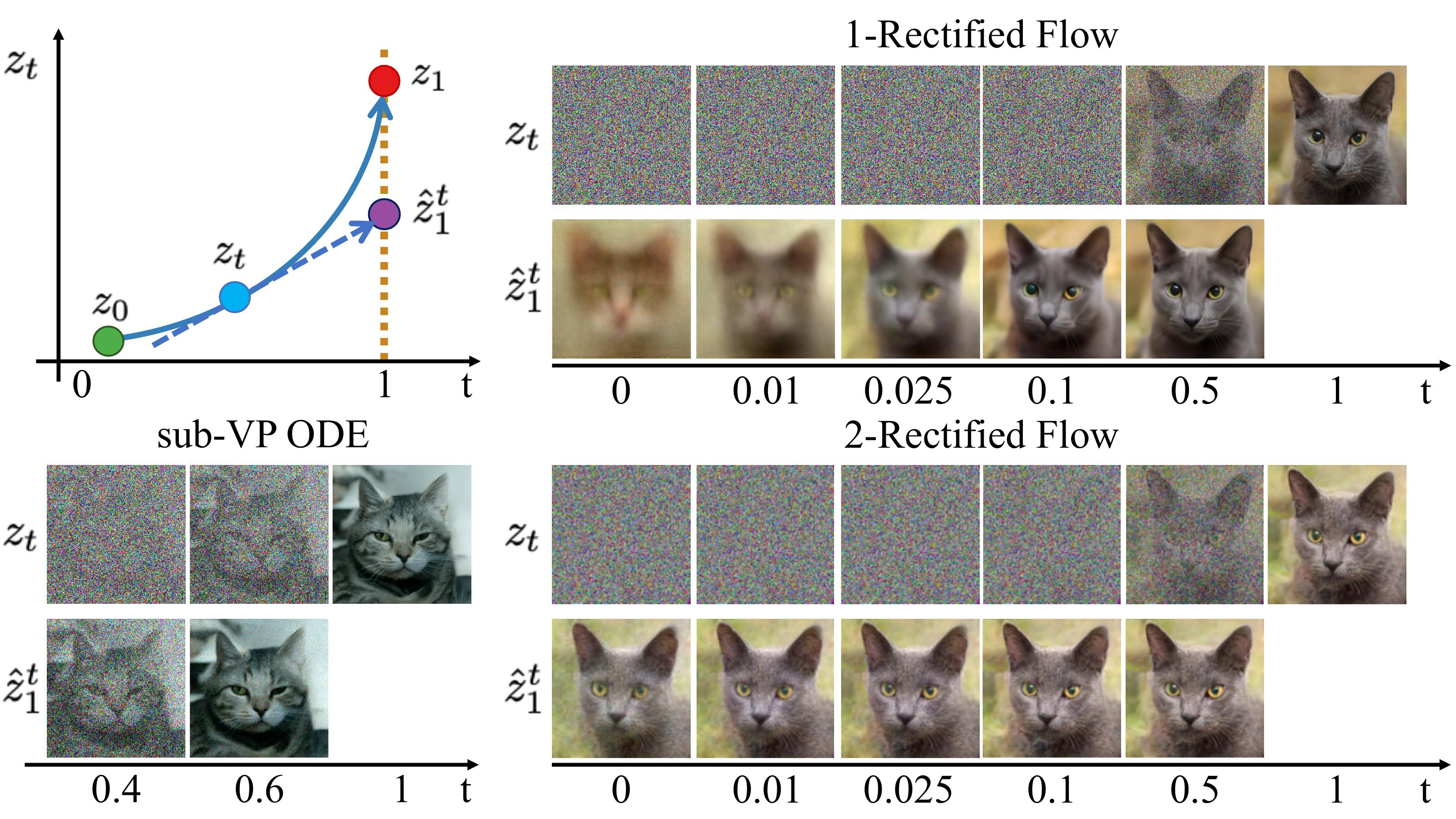
Reflow: Fast Generation with Straight Flows

Denote the rectified flow $Z = { Z_t : t \in [0, 1] }$ induced from $(X_0, X_1)$ by:

$$ Z = \text{Rectflow}((X_0, X_1)). $$

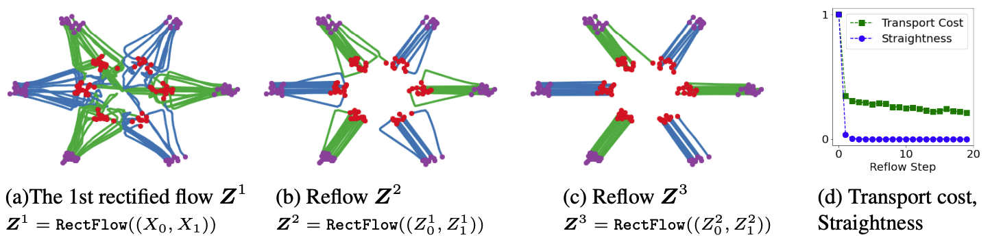
Applying the $\text{Rectflow}(\cdot)$ operator recursively yields a sequence of rectified flows:

$$ Z^{k+1} = \text{Rectflow}((Z_0^k, Z_1^k)), $$

where $(Z_0^0, Z_1^0) = (X_0, X_1)$. Here, $Z^k$ is the $k$-th rectified flow, induced from $(X_0, X_1)$.

In practice:

• We sample $(Z_0^k, Z_1^k)$ from the current $k$-th rectified flow,
• Then retrain a new rectified flow from these samples,
• Each step makes the flow paths straighter.

Why This Matters?

Besides lowering transport cost, this “reflow” process has an important side effect:

• It straightens the paths of rectified flows.
• As $k$ increases, the paths of $Z^k$ become increasingly straight.

Key Properties

The straightness of a flow $Z$ can be measured by:

$$ s(Z) = \int_0^1 \mathbb{E} \left[ | Z_1 - Z_0 - v(Z_t, t) |^2 \right] dt, $$ where:

• $S(Z) = 0$ corresponds to perfectly straight paths.
• After $k$ iterations, we have:

$$ \min_{k \leq K} S(Z^k) = O(1/K). $$ Computational Advantage: Flows with nearly straight paths are computationally efficient:

• They have minimal discretization error.
• If the ODE $dZ_t = v(Z_t, t) dt$ has straight paths, then:

$$ Z_t = Z_0 + t v(Z_0, 0), $$

Meaning: the ODE can be solved exactly with just a single Euler step!

This addresses the slow inference bottleneck of traditional ODE/SDE models. Thus, reflow enables training one-step generative models (like GANs or VAEs) using ODE flows.

In this blog, we took a deep dive into the world of flows — exploring what a flow is, understanding normalizing flows, learning about flow matching, and diving into conditional and marginal probability paths and vector fields. We also unpacked rectified flows in detail. Altogether, this has helped us build a strong theoretical foundation and intuition around flows. In the next blog, we’ll shift gears and explore different flow-based models and their architectures.

References

1. Flow Matching Guide and Code- Y. Lipman
2. Flow Matching for Generative Modeling - Y. Lipman
3. Normalizing Flows: An Introduction and Review of Current Methods - Ivan Kobyzev
4. Flow Straight and Fast: Learning to Generate and Transfer Data with Rectified Flow - Xingchao Liu
5. Scaling Rectified Flow Transformers for High-Resolution Image Synthesis - Patrick Esser - Stability AI
6. Flow-based Deep Generative Models - Lilian Weng