The next frontier of large language model optimization isn’t architectural - it’s infrastructural. We’ve squeezed what we can from model design; now, inference efficiency is dictated by how we map computation to hardware. The challenge is executing them with minimal memory movement, maximal kernel fusion and predictable latency across heterogeneous batches. Every inefficiency (redundant projection, scattered memory access, unaligned kernels) compounds at scale. The gap between theoretical FLOPs and delivered throughput is now a systems problem.
FlashInfer is a response to kernel-level fragmentation in that gap. Rather than forcing every inference framework to reimplement attention from scratch, it provides a unified kernel interface optimized for modern GPU execution patterns. Its design is unapologetically focused: efficient paged KV-cache for scattered memory layouts, multi-backend dispatch to vendor-optimized kernels when available, sparse attention patterns for long-context scenarios, and a clean API that lets frameworks control scheduling while FlashInfer handles execution.
This blog dissects FlashInfer as a system: how its abstractions expose structure rather than hide it, how it redefines attention as a pipeline of specialized kernels, and how it embodies the principle that efficiency is achieved through representation - of data, of memory and of computation.
FlashInfer as a Unified Kernel Interface
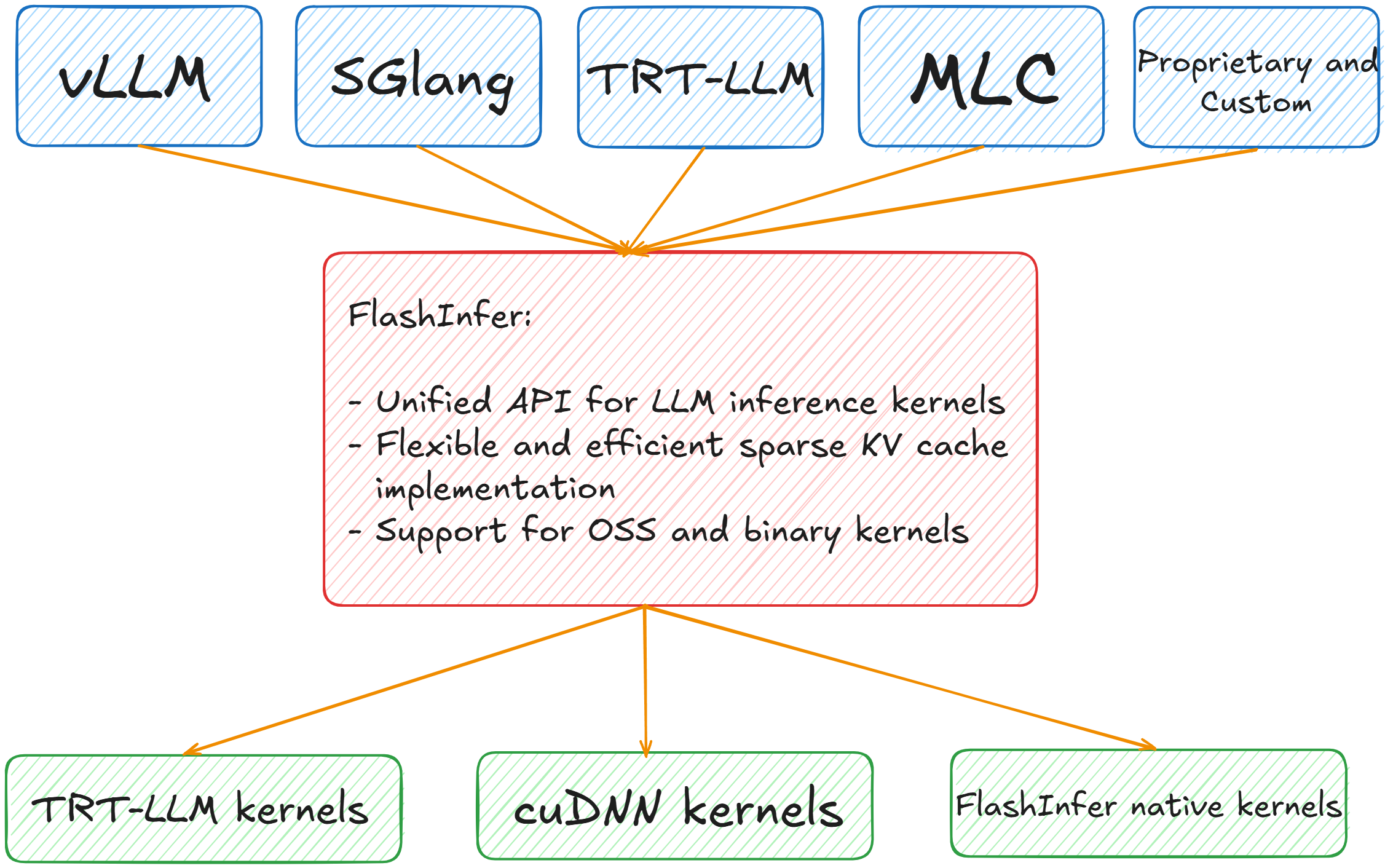
FlashInfer positions itself as an intermediate layer between inference frameworks and the actual kernel implementations that execute on GPUs. Rather than each framework implementing its own attention kernels or choosing a single backend, FlashInfer provides a unified API that abstracts over multiple kernel sources. The architecture is straightforward: frameworks like vLLM, SGLang, TRT-LLM, MLC-LLM, and proprietary systems integrate with FlashInfer’s API at the top, while FlashInfer routes those calls to appropriate kernel implementations at the bottom (whether TensorRT-LLM kernels, cuDNN kernels, or FlashInfer’s own native implementations). This design provides frameworks with flexibility in kernel selection while maintaining a consistent interface. A framework doesn’t need to hard-code dependencies on specific kernel libraries; instead, it expresses attention operations through FlashInfer’s API, and the actual kernel used can vary based on hardware capabilities, model characteristics, or runtime configuration.
Unified KV-Cache Format and Dynamic-Aware Runtime
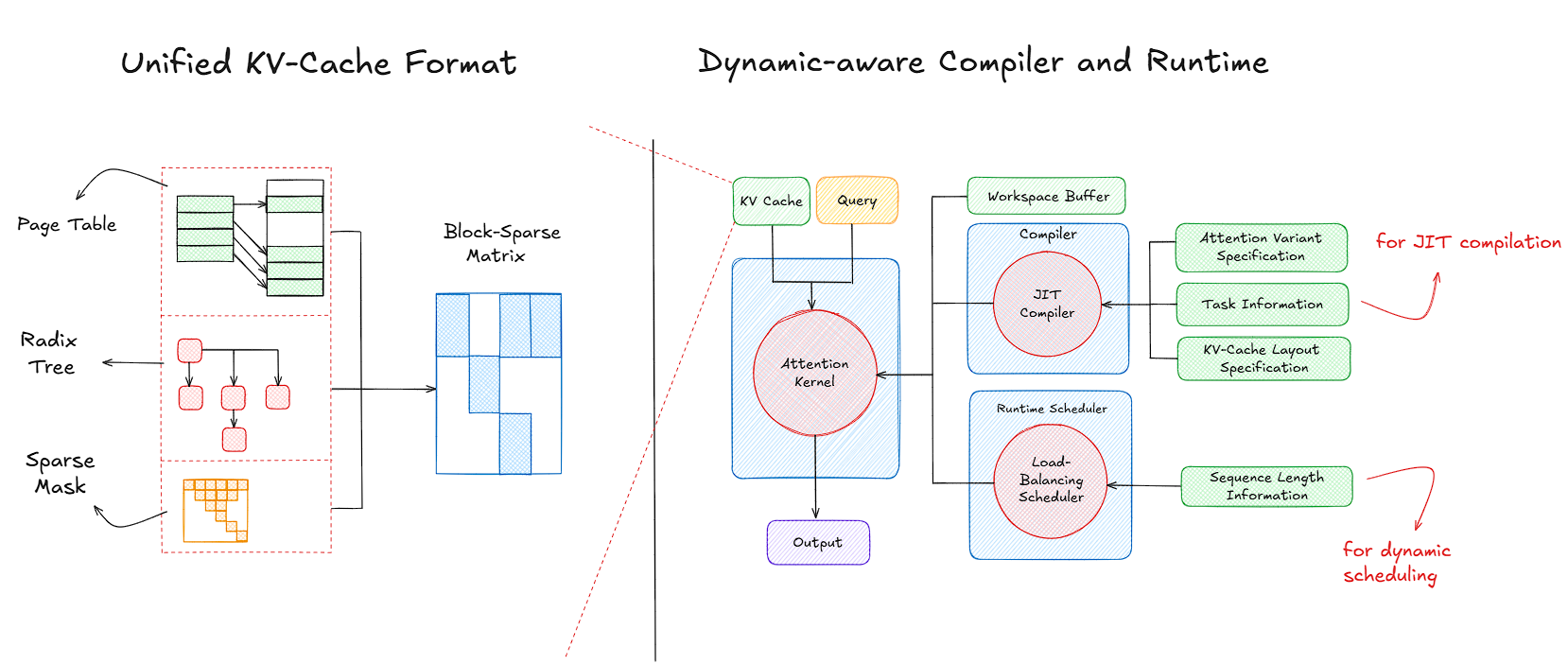
When building high-performance inference engines for large language models, one of the hardest challenges is handling dynamic workloads - workloads where sequence lengths vary across requests, attention patterns differ across models, and memory layouts shift depending on the framework you’re integrating with. FlashInfer approaches this problem by introducing two key components: a unified KV-cache format that can represent multiple caching strategies under one abstraction, and a dynamic-aware compiler and runtime that compiles and schedules attention kernels adaptively at runtime. Together, these two components form the foundation of FlashInfer’s ability to achieve high throughput without sacrificing flexibility.
The Unified KV-Cache Format
At its core, the KV cache is a memory structure storing the key and value tensors produced during autoregressive decoding. Each new token appends to this cache, and every subsequent token’s attention must reference the entire history. In practice, however, this seemingly simple mechanism becomes a bottleneck - both because memory grows linearly with sequence length and because access patterns vary widely across inference scenarios.
The KV cache fundamentally serves as a memory buffer that retains key and value tensors generated during autoregressive token generation. As each token is produced, its corresponding K/V representations are stored, allowing subsequent tokens to compute attention over the accumulated context without redundant computation. While conceptually straightforward, this mechanism creates practical challenges: memory consumption scales linearly with context length, and how the cache is accessed differs significantly depending on the inference workload.
FlashInfer addresses this through a unified KV-cache format that treats the cache as a block-sparse tensor structure. Here, each block represents a contiguous chunk of tokens within the sequence. Rather than hardcoding assumptions about the underlying storage backend (whether it’s vLLM’s page-based allocation, a single contiguous memory buffer, or another scheme) the unified format provides a consistent abstraction layer. Blocks are independently addressable, sparsity metadata explicitly describes which portions of the cache are active, and this structural information is exposed to the runtime for optimized kernel dispatch. The result: FlashInfer kernels can operate seamlessly across diverse caching strategies - dense layouts, paged memory, structured sparse attention patterns - without requiring backend-specific code paths.
Block Sparse Row (BSR) Format for Efficient Sparse Matrix Storage
Sparse matrices appear frequently in machine learning systems, from attention masks in transformers to adjacency matrices in graph neural networks. While sparsity offers opportunities for memory and compute savings, naively storing only non-zero elements can introduce significant indexing overhead. Traditional element-wise sparse formats (like CSR or COO) introduce irregular memory access and branching overhead, which GPUs handle poorly. The Block Compressed Row (BSR) format offers a more structured alternative, one that leverages block-level regularity to preserve sparsity benefits while maintaining efficient memory locality.
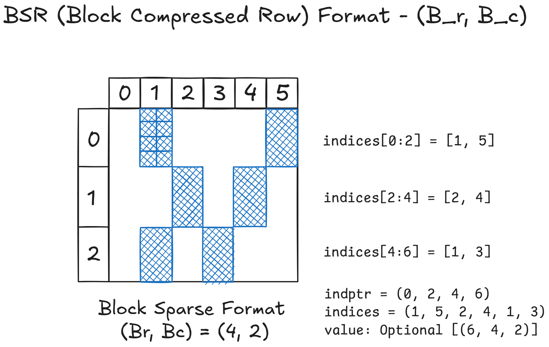
At a high level, the BSR format partitions the matrix into fixed-size dense blocks of shape $(Br, Bc)$ where $Br$ is the number of rows and $Bc$ is the number of columns in each block. Instead of storing every individual non-zero entry, BSR stores entire non-zero blocks along with their corresponding column indices. This representation is particularly suitable when the sparsity pattern exhibits structured locality, as is common in attention maps with banded or sliding-window structures.
The diagram above illustrates a block-sparse matrix divided into 3 block rows and 6 block columns. Each non-zero region (shown in blue) corresponds to a dense block of shape $(Br,Bc)=(4, 2)$. In total, the matrix contains 6 non-zero blocks spread across the three block rows. To represent a block-sparse matrix compactly, the Block Compressed Row (BSR) format relies on three key arrays: indptr, indices, and values. The indptr array, short for index pointer, specifies where each block row begins and ends within the indices array. For example, given indptr = [0, 2, 4, 6], we know that block row 0 spans entries indices[0:2], block row 1 spans indices[2:4], and block row 2 spans indices[4:6]. This effectively partitions the indices array according to the number of non-zero blocks per row.
The indices array stores the column indices of non-zero blocks within each block row. In this case, indices = [1, 5, 2, 4, 1, 3] tells us that block row 0 contains non-zero blocks in columns 1 and 5, block row 1 contains non-zero blocks in columns 2 and 4, and block row 2 contains non-zero blocks in columns 1 and 3. Together, indptr and indices provide a complete structural map of where non-zero blocks reside, without storing any actual numerical values.
Finally, the values array (optional) holds the actual data for each non-zero block. Each entry in values corresponds to a small dense submatrix of fixed size $(Br, Bc)$, such as $(4, 2)$. The blocks are stored in the same order as specified by the indices array, ensuring that the position of each block can be reconstructed efficiently during computation. This separation between structure (indptr and indices) and data (values) makes BSR both memory-efficient and GPU-friendly.
Page Attention as a Block-Sparse Matrix
In large-scale inference, the KV cache holds the keys and values for all tokens generated so far. When serving batched requests, each request may have different sequence lengths, and thus different cache footprints. To support dynamic batching without wasting compute on padding, paged attention partitions the cache into fixed-size memory pages, treating each page as a unit block for addressing and computation.
This design enables FlashInfer to reinterpret the attention operation as a block-sparse matrix multiplication, where the query corresponds to one dimension (rows) and the paged KV-cache to another (columns). The sparsity arises because not every query attends to every page (only a subset of pages corresponding to that request’s context).
1. Logical KV-Cache Block
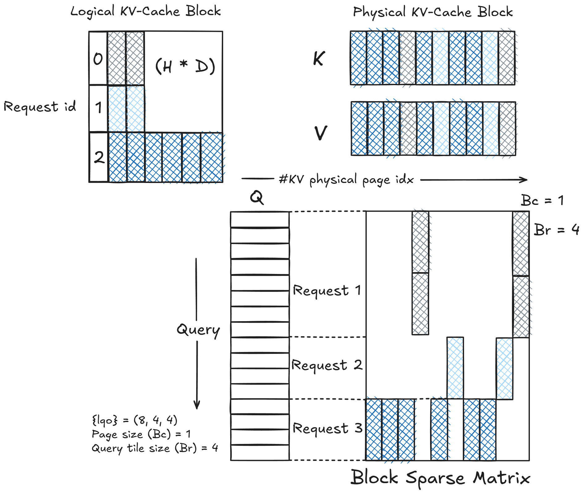
The top-left portion of the diagram represents the logical view of the KV cache across multiple requests. Each row corresponds to a request ID, and each column corresponds to the feature dimension (head × hidden size, $H×D$). Only some portions are filled (shaded), reflecting that different requests have different active tokens or pages.
This logical layout is conceptual (it doesn’t map directly to physical memory). The challenge is to convert this irregular structure into a hardware-aligned layout suitable for GPU computation.
2. Physical KV-Cache Block
The top-right part shows how keys (K) and values (V) are stored physically.
Instead of continuous sequences per request, they are organized as pages: each page representing a fixed-size slice of the KV cache. This is akin to virtual memory: the runtime can map logical positions to physical pages efficiently. For example, pages may have size $Bc=1$, meaning each block column corresponds to one page of KV entries.
These physical pages form the columns of the eventual block-sparse matrix.
Requests that share similar cache sizes or attention spans will have non-zero entries aligned in the same columns.
3. Query Tiles and Block Layout
The bottom portion of the diagram illustrates the core structure of the computation: a block-sparse matrix representing the attention operation. Instead of operating over a dense query–key matrix, the attention is reformulated as a tiled computation, where both queries and KV-cache entries are partitioned into fixed-size blocks.
In this structure, the rows correspond to query tiles, each containing a fixed number of queries (here, the tile size is $Br=4$). This means each block row represents a group of four consecutive queries, processed together for efficiency. Similarly, the columns correspond to KV pages, each with a fixed capacity of cached keys and values, with a page size of $Bc=1$. Each block column thus represents a discrete, memory-aligned unit of the KV cache. The non-zero blocks (the shaded regions in the diagram) represent active interactions (those query tiles that actually attend to specific KV pages). Blocks that remain unshaded indicate inactive regions, meaning the corresponding queries do not attend to those pages and their computations can be safely skipped. This selective computation gives rise to a block-sparse matrix structure.
Each request occupies a contiguous set of rows within this matrix, reflecting the queries associated with that specific request. For example, Request 1’s queries attend to only a few KV pages, leading to a sparse row segment with limited active blocks. In contrast, Request 3 attends to more KV pages, resulting in a denser region with several active blocks. This per-request tiling ensures that different sequence lengths can coexist efficiently in the same batch.
The overall sparsity pattern is determined by the sequence lengths of individual requests and the paging metadata derived from their KV-cache layouts. Since not every query–page pair is valid, the matrix naturally exhibits a structured sparsity, forming a block-sparse attention mask. The runtime computes only the active blocks, while skipping the inactive ones, significantly reducing redundant computation.
KV-Cache Storage and Tensor Core Compatibility
One of the key challenges in executing sparse attention efficiently on GPUs lies in how KV-cache data is stored and accessed during matrix multiplications. Sparse data structures often break the memory alignment and coalescing patterns that Tensor Cores rely on for high throughput. FlashInfer overcomes this by using a block-sparse row format that preserves contiguity in the last dimension, allowing the system to retain Tensor Core compatibility while operating on sparse rows and columns.
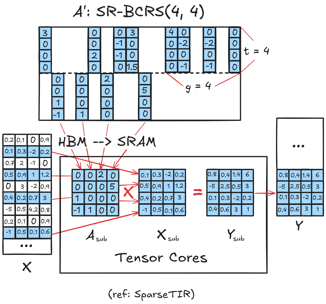
The FlashInfer kernel executes the attention computation in two memory stages:
i) Loading from Global Memory (HBM) to Shared Memory (SRAM):
Rows are fetched from global memory in their sparse form, where each row may contain only a subset of active blocks. During this stage, FlashInfer loads only the non-zero blocksinto shared memory, transforming them into a dense layout ready for tensor core consumption. Because each block’s last dimension is contiguous, memory accesses remain coalesced, minimizing bandwidth waste.
ii) Compute on Tensor Cores:
Once in shared memory, these dense tiles are fed directly into Tensor Cores. The kernel performs standard dense GEMM (matrix multiply) operations on these tiles, producing partial outputs. Importantly, since only non-zero blocks are loaded, no compute cycles are wasted on zero regions achieving both data sparsity and compute regularity.
This workflow allows FlashInfer to exploit the hardware efficiency of dense tensor operations, while still reaping the memory and compute savings of sparsity.
The critical condition enabling this design is that the last dimension of each sub-block remains contiguous in memory. This contiguity ensures:
- Coalesced global memory loads: threads fetch consecutive elements in one transaction.
- Aligned shared memory storage: blocks map cleanly to SRAM banks.
- Tensor Core readiness: operands are pre-packed in the required layout.
Memory Hierarchy and Execution
The above diagram shows how the computation unfolds:
- From HBM (global memory), sparse sub-blocks of $A^`$ (e.g., the KV cache) are loaded into SRAM (shared memory).
- Each block, $A_{\text{sub}}$, is multiplied with the corresponding tile $X_{\text{sub}}$ (e.g., query fragments), producing partial outputs $Y_{\text{sub}}$.
- Tensor Cores handle these multiplies efficiently as dense operations, and results are accumulated into the output buffer $Y$.
This design allows FlashInfer to run sparse attention as a sequence of dense tile multiplications, orchestrated via runtime scheduling that maps only active tiles to GPU compute threads.
Divide and Conquer Attention over Shared and Unique KV-Caches
In large-scale LLM serving, multiple requests often share overlapping context tokens - especially when decoding from similar prompts or during batch inference in applications like retrieval-augmented generation. A naive approach processes each request independently, reloading identical key-value (KV) pairs multiple times from global memory. This wastes bandwidth and compute, especially since global memory is the slowest component in the GPU memory hierarchy. FlashInfer introduces a divide-and-conquer strategy that separates shared and unique KV segments, dramatically improving memory efficiency.
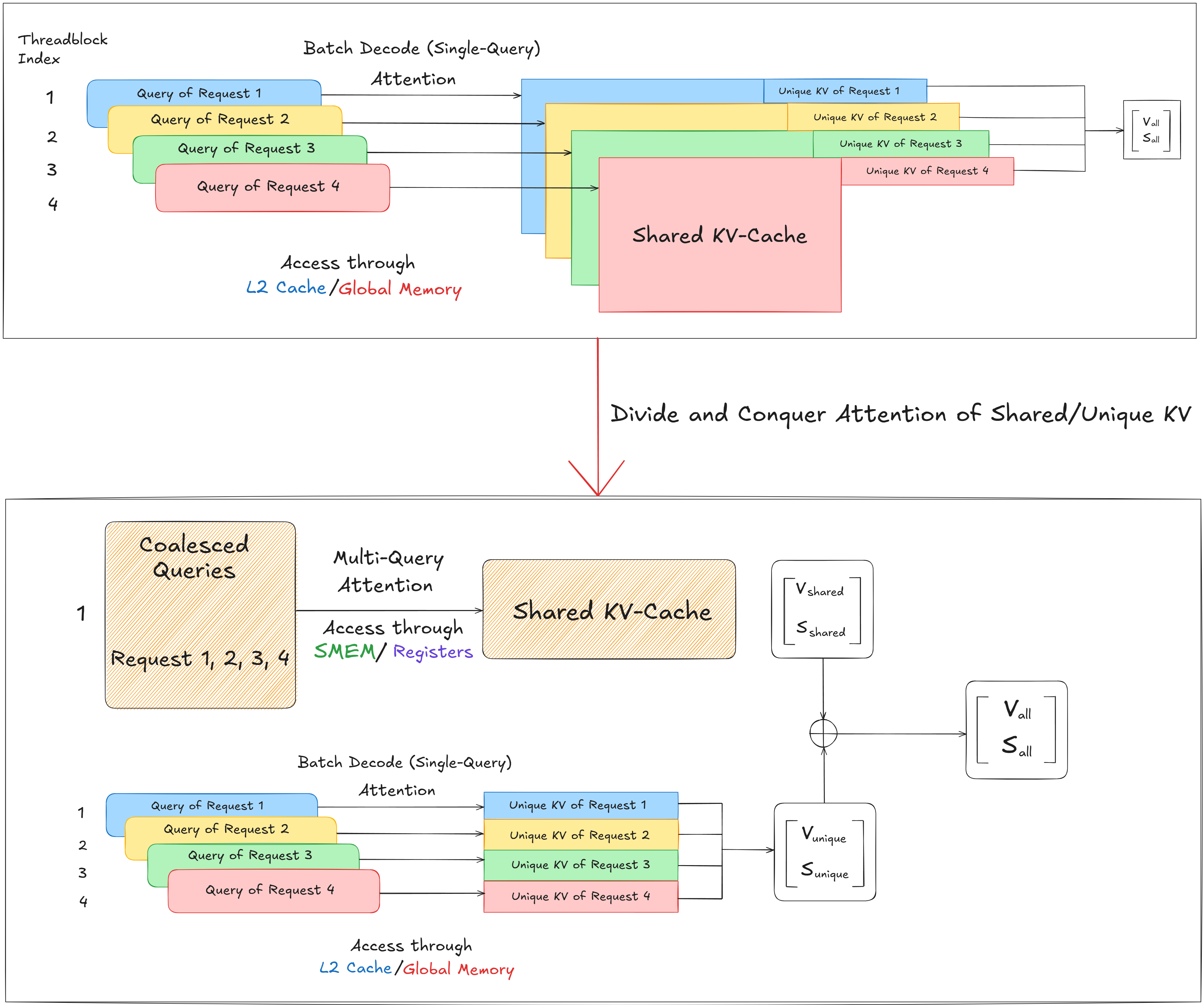
Baseline: Batch Decode with Single-Query Attention
In the traditional batch decode setup, each thread block handles a single query from a different request. Every query performs attention over its own KV-cache, even if portions of those caches overlap. Access to the shared KV regions happens repeatedly across requests, with each thread block loading the same data from L2 cache or global memory. This model achieves functional correctness but incurs high memory traffic and redundant compute, since shared tokens are reloaded and recomputed multiple times.
FlashInfer restructures the computation into two distinct phases:
i) Shared KV Phase (Multi-Query Attention):
All queries across requests that reference the same shared KV tokens are grouped and processed together. These coalesced queries perform attention jointly over the shared KV-cache, leveraging SMEM (shared memory) and registers for fast access. Since shared tokens are loaded only once, this phase maximizes data reuse and exploits high-bandwidth memory tiers (registers: ~600 TB/s, shared memory: ~19 TB/s).
ii) Unique KV Phase (Single-Query Attention):
Each request then independently processes its unique KV segments — tokens that are not shared with others. These segments are smaller and sparse, so they are fetched directly from L2 cache or global memory. Since unique tokens vary per request, these are handled in parallel by individual thread blocks using standard attention kernels.
The results from both phases - shared attention outputs $(V_{\text{shared}}, S_{\text{shared}})$ and unique attention outputs$(V_{\text{unique}}, S_{\text{unique}})$ - are combined to form the final result:
$$(V_{\text{all}}, S_{\text{all}}) = (V_{\text{shared}} + V_{\text{unique}}, ; S_{\text{shared}} + S_{\text{unique}})$$
This two-phase decomposition significantly improves throughput and cache utilization.
This design is deeply memory hierarchy-aware:
- Registers and shared memory are used for the shared KV phase to maximize data locality and reuse.
- L2 cache and global memory are used for unique KVs, minimizing contention and allowing concurrent memory access across requests.
JIT Compiler: Dynamic Specialization for Attention Variants
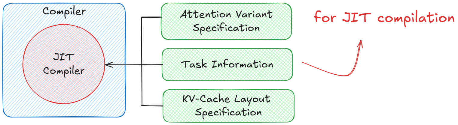
A defining feature of FlashInfer is its Just-In-Time (JIT) Compiler, designed to dynamically specialize attention kernels for a wide variety of attention variants, problem shapes, and KV-cache layouts. Unlike static kernel implementations that hardcode specific operations, FlashInfer’s JIT layer exposes a programmable interface that allows users to define and fuse custom operations directly into the kernel - all while preserving CUDA/Tensor Core efficiency! The JIT Compiler operates as a meta-scheduler: at runtime, it examines the current attention configuration (variant, sequence length, sparsity, layout) and compiles an optimized kernel tailored to those parameters. This makes the system both flexible (supporting new attention mechanisms) and highly performant (avoiding general-purpose overheads).
FlashInfer’s JIT system enables attention customization using a set of user-defined functors (lightweight functions that specify how queries, keys, and logits should be transformed). Inspired by FlexAttention and AITemplate (Meta), this design allows researchers and practitioners to inject new attention mechanisms without rewriting CUDA code. Three key function classes define the behavior:
QueryTransform/KeyTransform– Transform query or key embeddings before computing attention scores (e.g., rotary position encoding).LogitsTransform– Modify attention logits post dot-product (e.g., adding ALIBI bias).LogitsMask– Apply a mask over logits to enforce structural constraints (e.g., causal masking, sliding windows, or custom sparsity).
This modular approach decouples the attention variant logic from the low-level CUDA execution, allowing the compiler to inline these operations into the fused kernel during JIT compilation.
With the JIT interface, FlashInfer supports a broad range of attention mechanisms by dynamically composing user-defined functors. It can implement ALIBI attention by adding relative position biases for efficient long-sequence modeling, RoPE attention by applying rotational position embeddings based on token offsets, and sliding window attention by restricting each query to attend only within a local range. It also supports sigmoid attention, introducing nonlinear transformations to the attention weights, and allows custom masks or biases for domain-specific patterns. By compiling these variants just-in-time, FlashInfer achieves the flexibility to express diverse attention types while maintaining the efficiency of highly optimized, fused kernels.
Compile-Time Scheduling and Kernel Specialization
The JIT compiler also handles compile-time scheduling, generating optimized kernels for different problem shapes and memory layouts. For instance:
- Dense / Contiguous KV-cache: Standard memory layout for sequential models.
- Sparse / Block-Sparse KV-cache: Used in paged attention or sparse memory systems.
During compilation, the JIT layer selects tiling strategies, loop unrolling, and tensor core fragment mappings appropriate to the workload. This ensures that every kernel instance maximizes GPU occupancy and minimizes data movement, regardless of sparsity or block size. Because kernels are compiled on demand, the system avoids bloating binary size with hundreds of precompiled variants - instead, it emits only the ones needed for the active workload.
Integration with FlashAttention Templates
Under the hood, FlashInfer’s JIT system builds on CUDA/Cutlass templates derived from FlashAttention-2/3. These templates define the core GEMM loops, memory hierarchies, and warp scheduling policies. The JIT compiler injects user-defined transformations and masks directly into these templates before compilation, producing a fused attention kernel specialized for both the variant and cache layout.
At runtime, FlashInfer’s JIT engine analyzes the current attention configuration (such as the variant, mask type, and cache format) then assembles the corresponding function graph and specializes a CUDA kernel with inline transformations. The compiled binary is cached for reuse, enabling the system to handle heterogeneous batches where each request may use a different attention type, all while sustaining extremely low launch latency in the microsecond range after the initial compilation.
Runtime Scheduler: Deterministic Load Balancing for Variable-Length Requests
In real-world LLM serving, incoming requests vary significantly in sequence length and KV-cache size. A naive scheduling strategy assigns one request per thread block, leading to load imbalance, underutilized GPU resources, and non-deterministic execution when requests differ in length. To solve this, FlashInfer introduces a cost-model-based runtime scheduler that dynamically partitions workloads into uniform tiles, distributes them evenly across thread blocks, and performs deterministic reductions to ensure correctness and reproducibility. This scheduler bridges the gap between heterogeneous input sequences and the homogeneous compute structure GPUs require for maximum throughput.
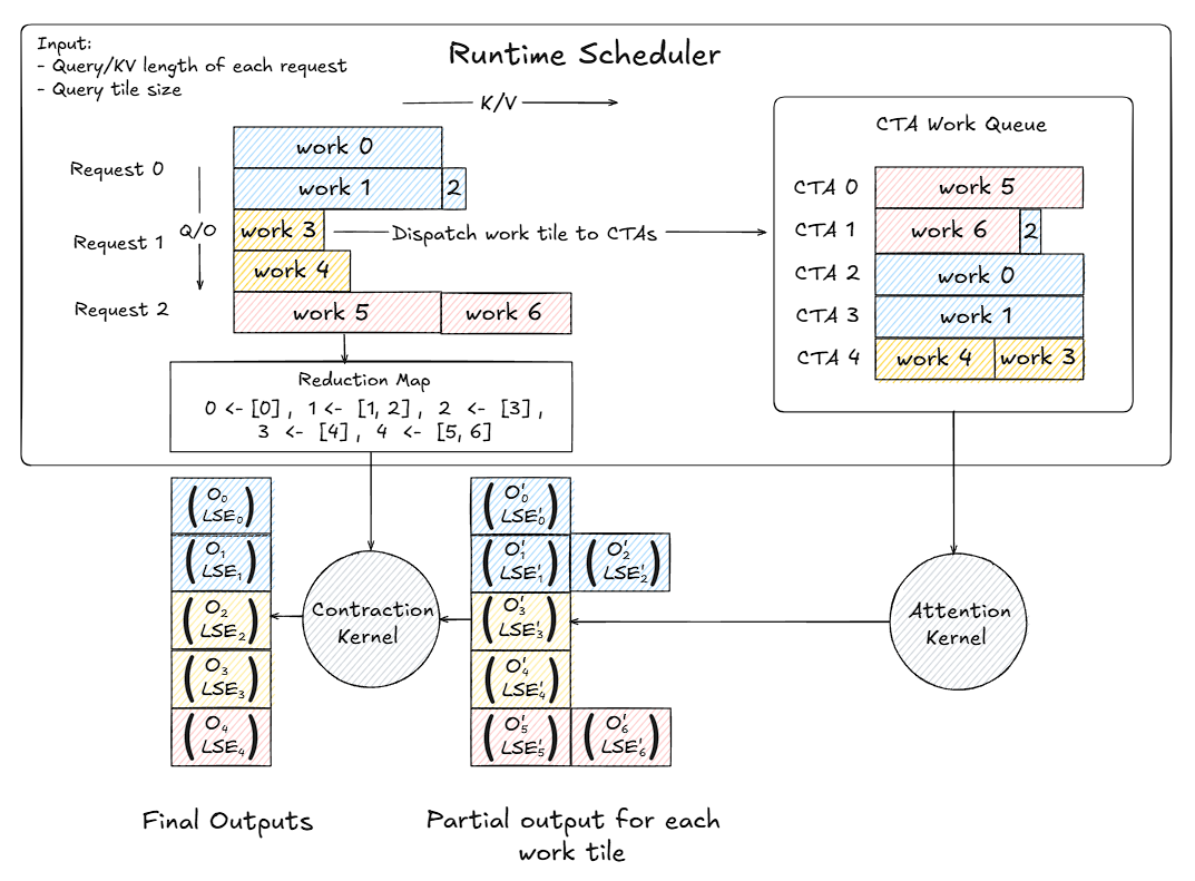
Cost-Model Partitioning
Each decoding step involves computing attention between a query tile and its corresponding key-value (KV) cache. Since requests have variable lengths, each has a different number of work units. The scheduler takes as input: a) the query length and KV length for each request and b) the query tile size (e.g., 64 or 128 tokens per tile). These parameters define a set of work tiles, each representing a unit of attention computation between a subset of queries and keys. The scheduler uses a cost model to partition each request’s workload into uniform tiles:
- Long sequences are divided into multiple tiles.
- Short sequences may fit into a single tile.
For example:
- Request 0 →
work 0,work 1,work 2 - Request 1 →
work 3,work 4 - Request 2 →
work 5,work 6
Each work tile corresponds to a fixed-size attention subproblem, ensuring consistent compute cost per tile. This tiling enables fine-grained scheduling, where the runtime can balance workload across all Cooperative Thread Arrays (CTAs).
Dispatch and Load Balancing
After partitioning, the scheduler assigns these work tiles to CTAs through a deterministic queue:
- Each CTA fetches work units in a predefined order, ensuring repeatable execution.
- The assignment balances the total number of tokens processed across CTAs, preventing idle compute units. For instance:
CTA 0→work 5,CTA 1→work 6,CTA 2→work 0, etc.
This results in even distribution and zero wave quantization - no idle “waves” of CTAs waiting for others to finish.
Execution Pipeline
Once dispatched, each CTA invokes the attention kernel on its assigned tile. The computation produces partial outputs - intermediate results containing the attention-weighted values and their corresponding log-sum-exp (LSE) normalization factors: $$(O_i’, LSE_i’) \text{ for each tile } i$$ These partial outputs are then sent to a contraction kernel for aggregation.
Deterministic Reduction
To ensure correctness, the scheduler maintains a reduction map linking tiles back to their parent request. Example: 0 ← [0], 1 ← [1, 2], 2 ← [3], 3 ← [4], 4 ← [5, 6]
This map instructs the contraction kernel to combine partial outputs belonging to the same request: $$(O_{\text{final}}, LSE_{\text{final}}) = \text{reduce}(O_i’, LSE_i’)$$This process is deterministic, meaning outputs are identical across runs regardless of GPU scheduling order. The contraction step fuses all partial results to produce final attention outputs for each request.
Integration with Compute Abstraction
This scheduling logic integrates seamlessly with FlashInfer’s compute abstraction, which follows an Init–Plan–Run model:
- Init: JIT-compile specialized kernels for each problem shape and attention variant.
- Plan: Use the runtime scheduler to partition workloads and determine the execution plan (load balancing, deterministic reduction).
- Run: Execute kernels according to the plan using CUDA graphs or
torch.compilefor maximum throughput.
This design amortizes compilation cost across multiple layers and decoding steps, achieving both dynamic adaptability and high efficiency.
Multi-Head Latent Attention (MLA) Decoding Kernel in FlashInfer
During my examination of FlashInfer’s kernel codebase, I found an implementation of the MLA (Multi-Head Latent Attention) decode kernel - a specialized kernel designed to efficiently execute latent attention by compressing KV caches and fusing matrix operations through the Matrix Absorption Trick. This caught my attention as it demonstrates how modern inference systems handle increasingly complex attention mechanisms at the kernel level.
Matrix Absorption Trick in MLA Decoding
In the standard Multi-head Latent Attention (MLA) design (as introduced in DeepSeekV2), decoding involves multiple sequential linear projections: one to map the hidden states into a low-rank query space (WᴰQ), another to expand queries into non-rotary and rotary subspaces (WᵁQ, WᵠR), and separate projections for compressed keys/values (WᵁK, WᵁV) before the final output projection (Wᴼ). Each step requires its own matrix multiplication and intermediate tensor, adding kernel overhead and memory traffic - especially problematic during token-by-token decoding.
The Matrix Absorption trick optimizes this by pre-composing these linear maps offline, leveraging the associative property of matrix multiplication. Instead of computing: $Q_{\text{nope}} = H \cdot W^{DQ} \cdot W^{UQ}, K_{\text{nope}} = C \cdot W^{UK}$ and then performing: $Q_{\text{nope}} \cdot K_{\text{nope}}^{\top}$ at runtime, the trick merges weights once: $$ W^{UQ_UK} = W^{UQ} \times W^{UK}$$ This fused matrix directly maps the low-rank query representation into a compressed latent space aligned with the KV cache, eliminating an intermediate projection. Similarly, the value projection and output projection are fused: $$ W^{UV_O} = W^{UV} \times W^{O} $$So after attention, the latent output is transformed to the final hidden dimension in one matmul. At runtime, decoding now involves:
- One projection for queries: $$ Q = H \cdot W^{DQ} $$
- One fused projection into the compressed latent space: $$ Q_{\text{latent}} = Q \cdot W^{UQ_UK} $$
- A single output projection using the pre-fused matrix: $$ O = A \cdot W^{UV_O} $$ where $A$ is the attention-weighted latent output.
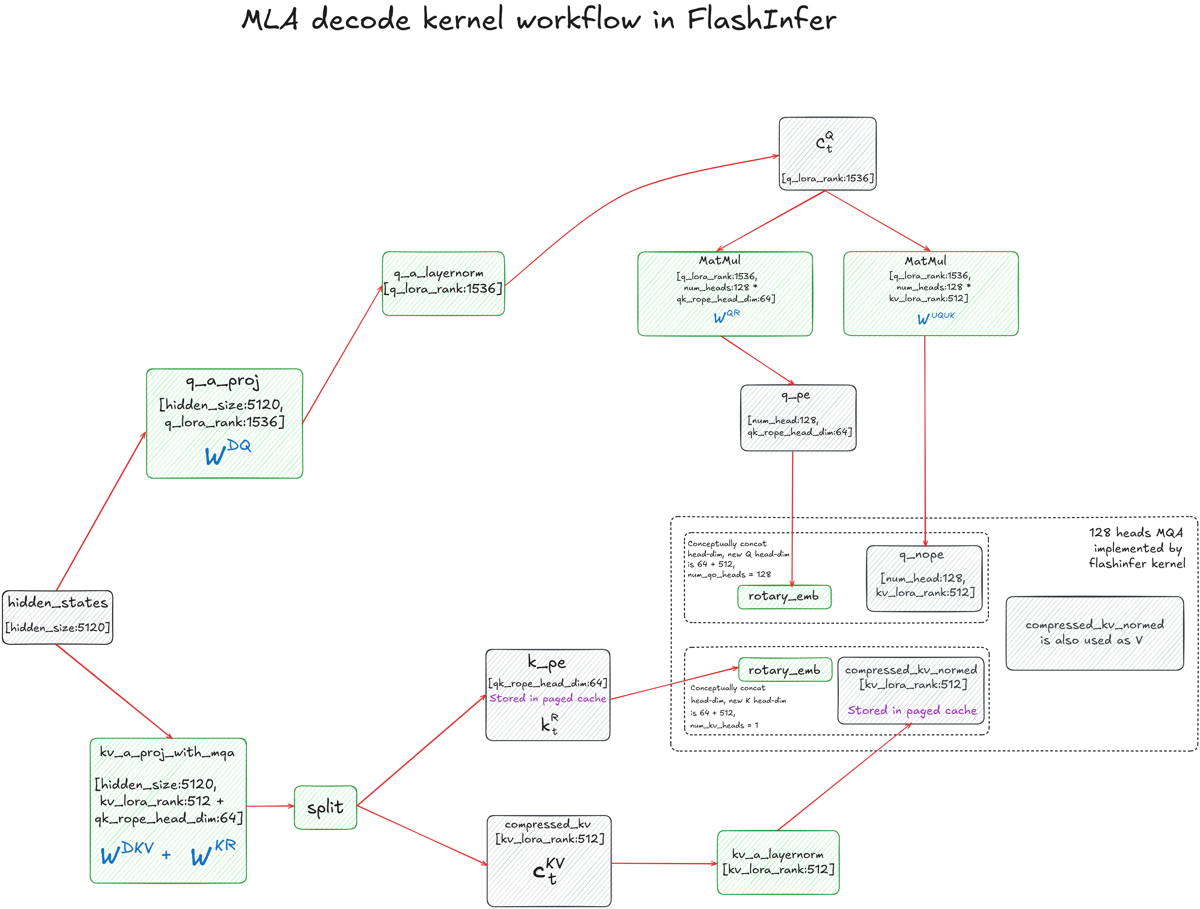
The MLA decode kernel workflow in FlashInfer implements an optimized version of Multi-head Latent Attention (MLA), designed to compress and efficiently utilize the KV cache during decoding. The process begins with the input hidden states (5120-dim), which are projected into a low-rank latent space through two main paths. The first path produces the query latent representation via $W^{DQ}$, followed by normalization with RMSNorm to yield $c_t^Q$. The second path generates a combined key-value representation through $W^{DKV} + W^{KR}$, which is then split into two components: $k_{pe}$, representing positional encodings, and compressed_kv, representing the compressed content used for both keys and values.
The query latent $c_t^Q$ is further decomposed into two parts: non-positional ($q_{nope}$) and positional ($q_{pe}$) components, computed via matrix multiplications with $W^{UQ}$ and $W^{QR}$, respectively. Similarly, the key-side positional encoding $k_{pe}$ is fused with $q_{pe}$ using rotary embeddings, embedding relative position information without explicit positional vectors. Both $q_{pe}$ and $k_{pe}$ are conceptually concatenated into higher-dimensional heads (64+512) for each of the 128 query heads. The attention computation is then carried out by FlashInfer’s 128-head MQA kernel, which reuses compressed_kv_normed as both K and V, achieving memory efficiency and reducing redundant projections.
The Matrix Absorption trick merges multiple linear layers into single composite matrices. This fusion precomputes the interactions between projection layers, effectively lowering the computational overhead during runtime. The absorbed matrices $W^{UQ_UK}$ and $W^{UV_O}$ enable decoding to operate directly in the latent space, minimizing FLOPs while maintaining accuracy. The final attention outputs are projected back to the original hidden dimension (5120) through the fused $W^{UV_O}$, completing a decoding pipeline that is both highly efficient and optimized for GPU memory access patterns.
By dissecting FlashInfer’s internals we gained a systems-level understanding of how LLM inference is evolving beyond naïve implementations toward hardware-saturating, latency-minimized, and throughput-optimized architectures. In essence, understanding FlashInfer gives you the blueprint for reasoning about how and why frameworks like vLLM schedule tokens the way they do, how SGLang optimizes radix-based serving, or how TensorRT fuses custom CUDA kernels for maximum efficiency. It’s a foundational step toward engineering the future of real-time, large-scale inference.